Dijkstra: Queue vs Priority Queue
Description
You are given a weighted undirected graph with V vertices (numbered 0 to V-1) and E edges, where every edge has a non-negative weight. You are also given a source vertex src.
Your task is to find the shortest path distances from the source vertex to every other vertex in the graph using Dijkstra's algorithm.
Return an array of size V where the i-th element represents the shortest distance from the source to vertex i.
This problem explores two different implementations of Dijkstra's algorithm:
- One using a simple linear scan (no priority queue) to select the next closest vertex.
- One using a priority queue (min-heap) to efficiently extract the minimum distance vertex.
Both produce the same correct result, but they differ significantly in time complexity.
Examples
Example 1
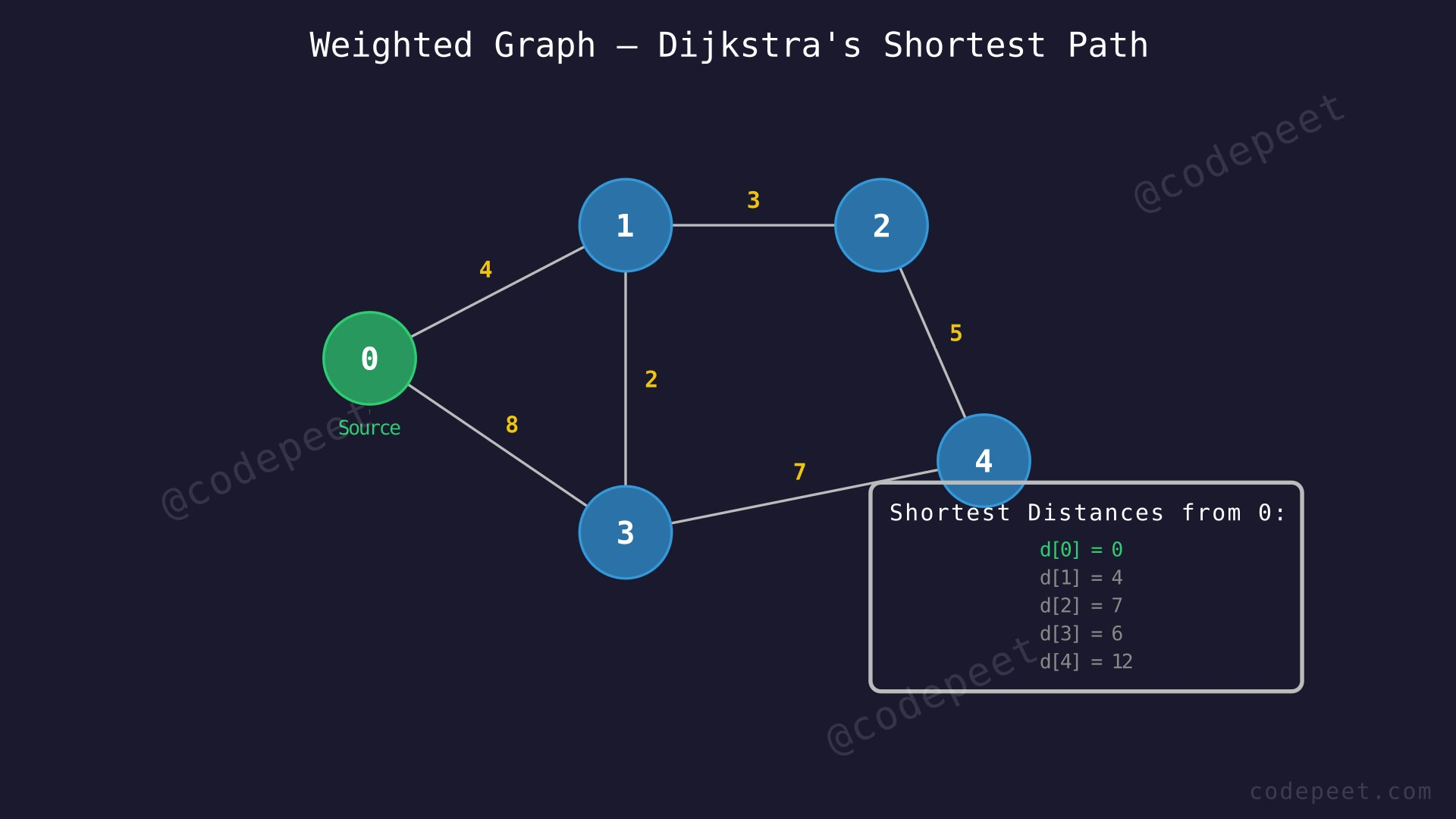
Input: V = 5, E = 6, src = 0
Edges: (0,1,4), (0,2,8), (1,2,3), (1,4,6), (2,3,2), (3,4,10)
Output: [0, 4, 7, 9, 10]
Explanation:
- dist[0] = 0: Source vertex, distance to itself is zero.
- dist[1] = 4: Direct edge 0→1 with weight 4.
- dist[2] = 7: Path 0→1→2 with total cost 4 + 3 = 7, which is shorter than the direct edge 0→2 with weight 8.
- dist[3] = 9: Path 0→1→2→3 with total cost 4 + 3 + 2 = 9.
- dist[4] = 10: Path 0→1→4 with total cost 4 + 6 = 10, which is shorter than 0→1→2→3→4 with cost 19.
Example 2
Input: V = 3, E = 3, src = 0
Edges: (0,1,1), (0,2,4), (1,2,2)
Output: [0, 1, 3]
Explanation:
- dist[0] = 0: Source vertex.
- dist[1] = 1: Direct edge 0→1 with weight 1.
- dist[2] = 3: Path 0→1→2 with cost 1 + 2 = 3 is shorter than direct edge 0→2 with weight 4. This demonstrates that Dijkstra finds indirect shorter paths.
Example 3
Input: V = 2, E = 1, src = 0
Edges: (0,1,5)
Output: [0, 5]
Explanation:
- dist[0] = 0: Source vertex.
- dist[1] = 5: Only one edge exists, so the shortest (and only) path is the direct edge with weight 5.
Constraints
- 1 ≤ V ≤ 10^5
- 0 ≤ E ≤ V × (V - 1) / 2
- 0 ≤ weight of each edge ≤ 10^6
- 0 ≤ src < V
- The graph is connected (every vertex is reachable from src)
- All edge weights are non-negative (no negative weights)
- No self-loops or multiple edges between the same pair of vertices
Editorial
Brute Force - Linear Scan
Intuition
Dijkstra's algorithm works on a simple principle: at every step, pick the unvisited vertex that is closest to the source, mark it as finalized, and then try to improve the distances to its neighbors.
The most straightforward way to implement this is without any special data structure. We maintain a distance array and a visited array. In each iteration, we scan through all vertices to find the unvisited one with the smallest distance. This is the "linear scan" approach — sometimes called using a "simple queue" because we are essentially searching through a flat list rather than using a smart data structure.
Think of it like a group of friends texting you their travel times to a meetup point. Without any sorting or priority system, you read through every message to find who arrives first. Then you process that person's connections and repeat. It works, but reading every message each time is slow when you have thousands of friends.
Step-by-Step Explanation
Let us trace through Example 1: V = 5, src = 0, edges: 0-1(4), 0-2(8), 1-2(3), 1-4(6), 2-3(2), 3-4(10).
Step 1: Initialize the distance array: dist = [0, ∞, ∞, ∞, ∞]. Source vertex 0 gets distance 0. All other vertices start at infinity. No vertices are visited yet.
Step 2: Scan all 5 vertices to find the unvisited vertex with minimum distance. Vertex 0 has dist=0, which is the smallest. Select vertex 0.
Step 3: Mark vertex 0 as visited. Check edge 0→1 (weight 4). Current path cost: dist[0] + 4 = 0 + 4 = 4. Since 4 < ∞ (dist[1]), update dist[1] = 4.
Step 4: Check edge 0→2 (weight 8). Path cost: 0 + 8 = 8. Since 8 < ∞ (dist[2]), update dist[2] = 8. Done processing vertex 0. dist = [0, 4, 8, ∞, ∞].
Step 5: Scan all 4 unvisited vertices {1, 2, 3, 4} to find the minimum. Compare distances: 4, 8, ∞, ∞. Vertex 1 with dist=4 is smallest. This linear scan cost O(V) work.
Step 6: Mark vertex 1 as visited. Check edge 1→2 (weight 3). Path cost: dist[1] + 3 = 4 + 3 = 7. Since 7 < 8 (dist[2]), update dist[2] = 7. Found a shorter path to vertex 2 through vertex 1.
Step 7: Check edge 1→4 (weight 6). Path cost: 4 + 6 = 10. Since 10 < ∞ (dist[4]), update dist[4] = 10. dist = [0, 4, 7, ∞, 10].
Step 8: Scan unvisited {2, 3, 4}. Distances: 7, ∞, 10. Vertex 2 with dist=7 is smallest. Mark vertex 2 as visited.
Step 9: Check edge 2→3 (weight 2). Path cost: 7 + 2 = 9. Update dist[3] = 9. dist = [0, 4, 7, 9, 10].
Step 10: Scan unvisited {3, 4}. Distances: 9, 10. Vertex 3 is smallest. Mark vertex 3. Check edge 3→4 (weight 10): 9 + 10 = 19. Since 19 > 10 (dist[4]), no update. The path through vertex 1 is already shorter.
Step 11: Only vertex 4 remains. Mark it as visited. No useful relaxations. Final result: dist = [0, 4, 7, 9, 10].
Dijkstra with Linear Scan — Processing All Vertices — Watch how each iteration requires scanning all unvisited vertices to find the minimum, then relaxes edges from the selected vertex.
Algorithm
- Create a distance array
dist[]of size V, initialize all values to infinity. Setdist[src] = 0. - Create a boolean array
visited[]of size V, all set to false. - Repeat V times:
a. Linear scan: Find the unvisited vertexuwith the smallestdist[u]by checking all V vertices.
b. Ifdist[u]is infinity, stop (remaining vertices are unreachable).
c. Markuas visited.
d. For each neighborvofuwith edge weightw:- If
vis not visited anddist[u] + w < dist[v], updatedist[v] = dist[u] + w.
- If
- Return
dist[].
Code
#include <vector>
#include <climits>
using namespace std;

class Solution {
public:
    vector<int> dijkstra(int V, vector<vector<pair<int,int>>>& adj, int src) {
        vector<int> dist(V, INT_MAX);
        vector<bool> visited(V, false);
        dist[src] = 0;

        for (int i = 0; i < V; i++) {
            // Linear scan: find unvisited vertex with minimum distance
            int u = -1;
            for (int j = 0; j < V; j++) {
                if (!visited[j] && (u == -1 || dist[j] < dist[u])) {
                    u = j;
                }
            }

            if (dist[u] == INT_MAX) break;
            visited[u] = true;

            // Relax all edges from u
            for (auto& edge : adj[u]) {
                int v = edge.first;
                int w = edge.second;
                if (!visited[v] && dist[u] + w < dist[v]) {
                    dist[v] = dist[u] + w;
                }
            }
        }
        return dist;
    }
};
import sys
class Solution:
def dijkstra(self, V: int, adj: list[list[tuple[int, int]]], src: int) -> list[int]:
dist = [sys.maxsize] * V
visited = [False] * V
dist[src] = 0
for _ in range(V):
# Linear scan: find unvisited vertex with minimum distance
u = -1
for j in range(V):
if not visited[j] and (u == -1 or dist[j] < dist[u]):
u = j
if dist[u] == sys.maxsize:
break
visited[u] = True
# Relax all edges from u
for v, w in adj[u]:
if not visited[v] and dist[u] + w < dist[v]:
dist[v] = dist[u] + w
return distimport java.util.*;
class Solution {
public int[] dijkstra(int V, List<List<int[]>> adj, int src) {
int[] dist = new int[V];
boolean[] visited = new boolean[V];
Arrays.fill(dist, Integer.MAX_VALUE);
dist[src] = 0;
for (int i = 0; i < V; i++) {
// Linear scan: find unvisited vertex with minimum distance
int u = -1;
for (int j = 0; j < V; j++) {
if (!visited[j] && (u == -1 || dist[j] < dist[u])) {
u = j;
}
}
if (dist[u] == Integer.MAX_VALUE) break;
visited[u] = true;
// Relax all edges from u
for (int[] edge : adj.get(u)) {
int v = edge[0], w = edge[1];
if (!visited[v] && dist[u] + w < dist[v]) {
dist[v] = dist[u] + w;
}
}
}
return dist;
}
}Complexity Analysis
Time Complexity: O(V²)
The algorithm runs V iterations. In each iteration, we perform a linear scan over all V vertices to find the unvisited vertex with the minimum distance. This scan alone takes O(V) per iteration. Over V iterations, the total scanning cost is V × O(V) = O(V²). The relaxation step across all iterations processes each edge at most once, adding O(E) total. Since E ≤ V², the dominant term is O(V²).
Space Complexity: O(V)
We use two arrays of size V: the distance array dist[] and the visited array visited[]. The adjacency list is part of the input and not counted as extra space.
Why This Approach Is Not Efficient
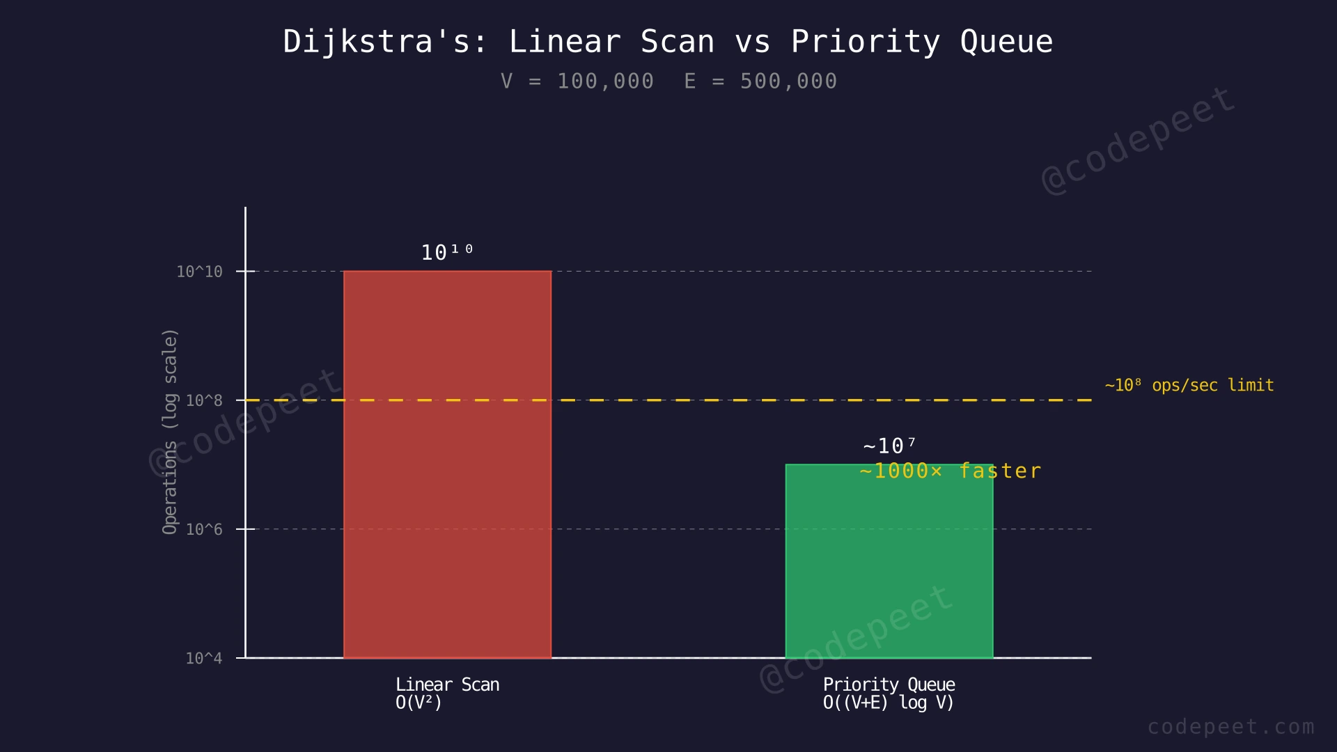
The linear scan approach has O(V²) time complexity because it scans all vertices to find the minimum distance vertex at every iteration. With V up to 10^5, this means up to 10^10 operations — far beyond the typical time limit of ~10^8 operations per second.
The bottleneck is the minimum-finding step. Each iteration, we ask: "Which unvisited vertex has the smallest distance?" Answering this by scanning all vertices is wasteful because we are repeating work. After a relaxation updates a few distances, only those few vertices might have changed — yet we re-examine all of them.
The key insight is: if we could maintain a data structure that always gives us the minimum distance vertex in O(log V) time instead of O(V), we would reduce the total time dramatically. A min-heap (priority queue) does exactly this — it keeps elements sorted by distance so extraction of the minimum costs O(log V), and insertion/update also costs O(log V).
This brings the overall complexity down from O(V²) to O((V + E) × log V), which is a massive improvement for sparse graphs where E is much smaller than V².
Optimal Approach - Priority Queue (Min-Heap)
Intuition
Instead of scanning every vertex to find the closest one, we use a priority queue (min-heap) to maintain the vertices sorted by their current shortest distance. The min-heap automatically gives us the vertex with the smallest distance at the top, so extracting it takes only O(log V) instead of O(V).
The algorithm is the same greedy Dijkstra logic — pick the closest unvisited vertex, finalize it, relax its edges — but the data structure makes it vastly faster.
One practical detail: when we discover a shorter path to a vertex, we push a new entry (new_distance, vertex) into the heap rather than updating the existing entry. This means the heap may contain stale (outdated) entries. When we pop an entry and its distance is larger than the already-known shortest distance for that vertex, we simply skip it. This is called lazy deletion, and it avoids the complexity of a decrease-key operation while keeping the algorithm correct.
Think of the priority queue like a hospital emergency room triage system. Instead of a nurse walking through every patient to find the most critical one (linear scan), patients are placed in a priority system where the most urgent case is always at the front. When a patient's condition changes, a new triage record is created. If an old record comes up but the patient has already been treated, it is simply discarded.
Step-by-Step Explanation
Let us trace through Example 1: V = 5, src = 0, edges: 0-1(4), 0-2(8), 1-2(3), 1-4(6), 2-3(2), 3-4(10).
Step 1: Initialize dist = [0, ∞, ∞, ∞, ∞]. Push (distance=0, vertex=0) into the min-heap. Heap: [(0,0)].
Step 2: Pop the minimum from the heap: (0, 0). This means vertex 0 with distance 0 is next to process.
Step 3: Relax edge 0→1 (weight 4). New distance: 0 + 4 = 4 < ∞. Update dist[1] = 4. Push (4, 1) into heap. Heap: [(4,1), (8,2)].
Step 4: Relax edge 0→2 (weight 8). New distance: 0 + 8 = 8 < ∞. Update dist[2] = 8. Push (8, 2) into heap. Heap: [(4,1), (8,2)].
Step 5: Pop minimum: (4, 1). Process vertex 1. The heap gave us vertex 1 in O(log n) — no scanning needed.
Step 6: Relax edge 1→2 (weight 3). New distance: 4 + 3 = 7 < 8. Update dist[2] = 7. Push (7, 2) into heap. Note: the old entry (8, 2) still exists in the heap — this is lazy deletion. Heap: [(7,2), (8,2), (10,4)].
Step 7: Relax edge 1→4 (weight 6). New distance: 4 + 6 = 10 < ∞. Update dist[4] = 10. Push (10, 4). Heap: [(7,2), (8,2), (10,4)].
Step 8: Pop minimum: (7, 2). Process vertex 2.
Step 9: Relax edge 2→3 (weight 2). New distance: 7 + 2 = 9 < ∞. Update dist[3] = 9. Push (9, 3). Heap: [(8,2), (9,3), (10,4)].
Step 10: Pop (8, 2). But dist[2] is already 7, which is less than 8. This is a stale entry — vertex 2 was already processed with a shorter distance. Skip it. This is the lazy deletion in action.
Step 11: Pop (9, 3). Process vertex 3. Relax edge 3→4 (weight 10): 9 + 10 = 19 > dist[4] = 10. No update — the existing path is shorter.
Step 12: Pop (10, 4). Process vertex 4. No useful updates.
Step 13: Heap is empty. Final distances: [0, 4, 7, 9, 10].
Dijkstra with Priority Queue — Efficient Minimum Extraction — Watch how the min-heap always provides the closest vertex instantly, and how stale entries are skipped via lazy deletion.
Algorithm
- Create a distance array
dist[]of size V, all initialized to infinity. Setdist[src] = 0. - Create a min-heap (priority queue). Push
(0, src)into it. - While the heap is not empty:
a. Pop the element(d, u)with the smallest distance from the heap.
b. Lazy deletion check: Ifd > dist[u], this is a stale entry — skip it.
c. For each neighborvofuwith edge weightw:- If
dist[u] + w < dist[v], updatedist[v] = dist[u] + wand push(dist[v], v)into the heap.
- If
- Return
dist[].
Code
#include <vector>
#include <queue>
#include <climits>
using namespace std;

class Solution {
public:
    vector<int> dijkstra(int V, vector<vector<pair<int,int>>>& adj, int src) {
        vector<int> dist(V, INT_MAX);
        // Min-heap storing (distance, vertex)
        priority_queue<pair<int,int>, vector<pair<int,int>>,
                       greater<pair<int,int>>> pq;

        dist[src] = 0;
        pq.push({0, src});

        while (!pq.empty()) {
            int d = pq.top().first;
            int u = pq.top().second;
            pq.pop();

            // Skip stale entries (lazy deletion)
            if (d > dist[u]) continue;

            // Relax all edges from u
            for (auto& edge : adj[u]) {
                int v = edge.first;
                int w = edge.second;
                if (dist[u] + w < dist[v]) {
                    dist[v] = dist[u] + w;
                    pq.push({dist[v], v});
                }
            }
        }
        return dist;
    }
};
import heapq
class Solution:
def dijkstra(self, V: int, adj: list[list[tuple[int, int]]], src: int) -> list[int]:
dist = [float('inf')] * V
dist[src] = 0
# Min-heap storing (distance, vertex)
pq = [(0, src)]
while pq:
d, u = heapq.heappop(pq)
# Skip stale entries (lazy deletion)
if d > dist[u]:
continue
# Relax all edges from u
for v, w in adj[u]:
if dist[u] + w < dist[v]:
dist[v] = dist[u] + w
heapq.heappush(pq, (dist[v], v))
return distimport java.util.*;
class Solution {
public int[] dijkstra(int V, List<List<int[]>> adj, int src) {
int[] dist = new int[V];
Arrays.fill(dist, Integer.MAX_VALUE);
dist[src] = 0;
// Min-heap storing [distance, vertex]
PriorityQueue<int[]> pq = new PriorityQueue<>(
(a, b) -> a[0] - b[0]
);
pq.offer(new int[]{0, src});
while (!pq.isEmpty()) {
int[] top = pq.poll();
int d = top[0], u = top[1];
// Skip stale entries (lazy deletion)
if (d > dist[u]) continue;
// Relax all edges from u
for (int[] edge : adj.get(u)) {
int v = edge[0], w = edge[1];
if (dist[u] + w < dist[v]) {
dist[v] = dist[u] + w;
pq.offer(new int[]{dist[v], v});
}
}
}
return dist;
}
}Complexity Analysis
Time Complexity: O((V + E) × log V)
Each vertex is popped from the priority queue at most once with its final shortest distance (stale entries are skipped in O(1)). Each pop operation costs O(log V). Each edge is examined at most once during relaxation, and each relaxation may push a new entry into the heap, costing O(log V). In total: V pops × O(log V) + E relaxations × O(log V) = O((V + E) × log V).
For sparse graphs where E is close to V, this is approximately O(V log V), which is dramatically faster than O(V²). For dense graphs where E approaches V², both approaches become similar since O(V² log V) can be slower than O(V²) — in that case, the linear scan approach is actually preferable.
Space Complexity: O(V + E)
The distance array uses O(V) space. The priority queue can hold at most O(E) entries in the worst case (one entry per edge relaxation), though typically it holds far fewer. The adjacency list uses O(V + E) as part of the input.