Graph Representation (C++)
Description
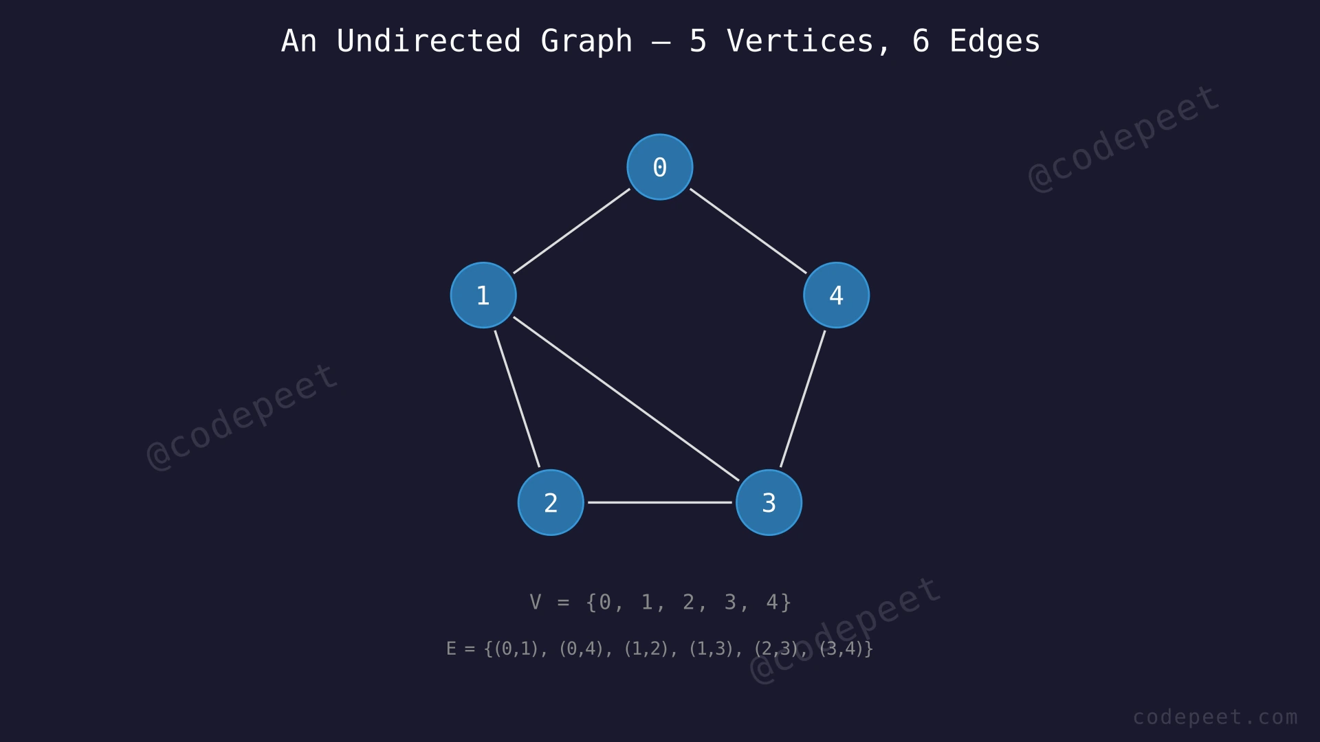
A graph is a non-linear data structure made up of two components:
- Vertices (Nodes): The individual entities in the graph, usually labeled with numbers (0, 1, 2, …) or letters.
- Edges: The connections between pairs of vertices. An edge links two vertices together.
Graphs are used to model relationships between objects — social networks (people connected by friendships), road maps (cities connected by roads), web pages (pages connected by hyperlinks), and countless other real-world systems.
Graphs come in two main flavors:
- Undirected Graph: Each edge has no direction. If vertex A is connected to vertex B, then B is also connected to A. Think of a two-way road.
- Directed Graph (Digraph): Each edge has a direction, going from one vertex to another. If there is an edge from A to B, it does not automatically mean there is an edge from B to A. Think of a one-way street.
Additionally, edges can carry weights — numeric values representing cost, distance, or capacity.
The fundamental question we address here is: How do we store a graph in memory so that a program can efficiently work with it? There are two primary representations:
- Adjacency Matrix — a 2D array where cell
[i][j]indicates whether an edge exists from vertexito vertexj. - Adjacency List — an array of lists where each list stores the neighbors of the corresponding vertex.
Given V vertices (numbered 0 to V−1) and E edges, implement both representations and understand their trade-offs.
Examples
Example 1
Input: V = 3, E = 3, edges = [(0,1), (0,2), (1,2)], undirected
Output (Adjacency Matrix):
0 1 1
1 0 1
1 1 0
Output (Adjacency List):
0 → [1, 2]
1 → [0, 2]
2 → [0, 1]
Explanation: This is a triangle graph — every vertex is connected to every other vertex. In the adjacency matrix, the entry at row i, column j is 1 if there is an edge between vertex i and vertex j, and 0 otherwise. The matrix is symmetric because the graph is undirected (an edge from 0 to 1 implies an edge from 1 to 0). In the adjacency list, each vertex stores the list of all vertices it is directly connected to.
Example 2
Input: V = 4, E = 4, edges = [(0,1), (1,2), (2,3), (3,0)], directed
Output (Adjacency Matrix):
0 1 0 0
0 0 1 0
0 0 0 1
1 0 0 0
Output (Adjacency List):
0 → [1]
1 → [2]
2 → [3]
3 → [0]
Explanation: This is a directed cycle: 0→1→2→3→0. Notice the adjacency matrix is not symmetric — mat[0][1] = 1 but mat[1][0] = 0, because the edge goes from 0 to 1, not the other way around. In the adjacency list, vertex 0 only has vertex 1 as a neighbor (outgoing edge), even though vertex 3 points back to vertex 0. The edge (3,0) appears in vertex 3's list, not in vertex 0's list.
Example 3
Input: V = 3, E = 3, edges = [(0,1,2), (0,2,5), (1,2,1)], undirected, weighted
Output (Adjacency Matrix):
0 2 5
2 0 1
5 1 0
Output (Adjacency List):
0 → [(1,2), (2,5)]
1 → [(0,2), (2,1)]
2 → [(0,5), (1,1)]
Explanation: In the weighted version, each edge carries a weight (cost, distance, etc.). The adjacency matrix stores the weight instead of 1. Entry mat[0][1] = 2 means the edge from vertex 0 to vertex 1 has weight 2. The adjacency list stores pairs of (neighbor, weight) instead of just the neighbor. Vertex 0's list [(1,2), (2,5)] means vertex 0 connects to vertex 1 with weight 2 and to vertex 2 with weight 5.
Constraints
- 1 ≤ V ≤ 10^5 (number of vertices)
- 0 ≤ E ≤ min(V × (V − 1) / 2, 10^5) for undirected graphs
- 0 ≤ E ≤ min(V × (V − 1), 10^5) for directed graphs
- 0 ≤ u, v < V (vertex indices are 0-based)
- Edge weights (if present): −10^9 ≤ w ≤ 10^9
- No self-loops (no edge from a vertex to itself) unless explicitly stated
- No duplicate edges in the input
Editorial
Adjacency Matrix
Intuition
The most straightforward way to represent a graph is with a two-dimensional table (matrix). Imagine a spreadsheet where both the rows and columns are labeled with vertex numbers. Each cell in this table answers one simple question: "Is there an edge between vertex i and vertex j?"
If the answer is yes, we put a 1 (or the edge weight) in that cell. If no, we put a 0.
Think of a classroom seating chart. You have a grid where each row is a student and each column is also a student. If two students are friends, you mark an X in the cell where their row and column intersect. This grid is your adjacency matrix.
For a graph with V vertices, we create a V × V matrix called adj. For each edge (u, v):
- Undirected graph: Set
adj[u][v] = 1ANDadj[v][u] = 1(friendship is mutual) - Directed graph: Set only
adj[u][v] = 1(a one-way connection) - Weighted graph: Store the weight instead of 1:
adj[u][v] = weight
In C++, the most natural way to create this matrix is using a 2D vector: vector<vector<int>> adj(V, vector<int>(V, 0)); — this gives us a V×V grid initialized to all zeros, ready to be filled as we process edges.
Step-by-Step Explanation
Let's build the adjacency matrix for Example 1: V = 3, edges = [(0,1), (0,2), (1,2)], undirected.
Step 1: Create a 3×3 matrix initialized with all zeros.
mat = [[0, 0, 0],
       [0, 0, 0],
       [0, 0, 0]]
Each cell mat[i][j] represents whether there is an edge from vertex i to vertex j.
Step 2: Process edge (0, 1). Set mat[0][1] = 1.
mat = [[0, 1, 0],
       [0, 0, 0],
       [0, 0, 0]]
Step 3: Since the graph is undirected, also set mat[1][0] = 1 (the mirror entry).
mat = [[0, 1, 0],
       [1, 0, 0],
       [0, 0, 0]]
Step 4: Process edge (0, 2). Set mat[0][2] = 1.
mat = [[0, 1, 1],
       [1, 0, 0],
       [0, 0, 0]]
Step 5: Mirror entry: set mat[2][0] = 1.
mat = [[0, 1, 1],
       [1, 0, 0],
       [1, 0, 0]]
Step 6: Process edge (1, 2). Set mat[1][2] = 1.
mat = [[0, 1, 1],
       [1, 0, 1],
       [1, 0, 0]]
Step 7: Mirror entry: set mat[2][1] = 1.
mat = [[0, 1, 1],
       [1, 0, 1],
       [1, 1, 0]]
Step 8: All 3 edges have been processed. The adjacency matrix is complete. Notice the matrix is symmetric along the diagonal (because the graph is undirected), and the diagonal itself is all zeros (no self-loops).
Building an Adjacency Matrix — Undirected Graph — Watch how each undirected edge fills two symmetric cells in the V×V matrix, gradually building the complete adjacency matrix.
Algorithm
- Read the number of vertices
Vand edgesE. - Create a
V × Vmatrix (2D array) initialized with all zeros. - For each edge
(u, v)in the input:- Set
mat[u][v] = 1(or the weight for weighted graphs). - If the graph is undirected, also set
mat[v][u] = 1(mirror entry). - If the graph is directed, only set
mat[u][v](one direction).
- Set
- The matrix is now ready. To check if an edge exists between vertices
iandj, simply readmat[i][j]. - To find all neighbors of vertex
i, scan the entire rowiand collect all columnsjwheremat[i][j] != 0.
Code
#include <bits/stdc++.h>
using namespace std;

int main() {
    int V, E;
    cin >> V >> E;

    // Create a V x V matrix initialized to 0
    vector<vector<int>> adj(V, vector<int>(V, 0));

    for (int i = 0; i < E; i++) {
        int u, v;
        cin >> u >> v;

        adj[u][v] = 1;
        adj[v][u] = 1; // Remove this line for a directed graph
    }

    // Print the adjacency matrix
    for (int i = 0; i < V; i++) {
        for (int j = 0; j < V; j++) {
            cout << adj[i][j] << " ";
        }
        cout << endl;
    }

    return 0;
}

// --- Weighted graph variant ---
// For weighted edges, read weight and store it instead of 1:
//
// for (int i = 0; i < E; i++) {
//     int u, v, w;
//     cin >> u >> v >> w;
//     adj[u][v] = w;
//     adj[v][u] = w; // Remove for directed
// }
def build_adjacency_matrix(V, edges, directed=False):
# Create a V x V matrix initialized to 0
adj = [[0] * V for _ in range(V)]
for u, v in edges:
adj[u][v] = 1
if not directed:
adj[v][u] = 1 # Mirror for undirected
return adj
# Read input
V, E = map(int, input().split())
edges = []
for _ in range(E):
u, v = map(int, input().split())
edges.append((u, v))
# Build and print the matrix
adj = build_adjacency_matrix(V, edges)
for row in adj:
print(" ".join(map(str, row)))
# --- Weighted graph variant ---
# For weighted edges, store the weight instead of 1:
#
# def build_weighted_matrix(V, edges, directed=False):
# adj = [[0] * V for _ in range(V)]
# for u, v, w in edges:
# adj[u][v] = w
# if not directed:
# adj[v][u] = w
# return adjimport java.util.Scanner;
public class Solution {
public static void main(String[] args) {
Scanner sc = new Scanner(System.in);
int V = sc.nextInt();
int E = sc.nextInt();
// Create a V x V matrix initialized to 0
int[][] adj = new int[V][V];
for (int i = 0; i < E; i++) {
int u = sc.nextInt();
int v = sc.nextInt();
adj[u][v] = 1;
adj[v][u] = 1; // Remove for directed graph
}
// Print the adjacency matrix
for (int i = 0; i < V; i++) {
for (int j = 0; j < V; j++) {
System.out.print(adj[i][j] + " ");
}
System.out.println();
}
}
}
// --- Weighted graph variant ---
// For weighted edges, read weight and store it:
//
// int u = sc.nextInt(), v = sc.nextInt(), w = sc.nextInt();
// adj[u][v] = w;
// adj[v][u] = w; // Remove for directedComplexity Analysis
Time Complexity:
-
Building the matrix: O(V² + E)
- Initializing the V×V matrix takes O(V²) time (every cell set to 0).
- Processing each of the E edges takes O(1) per edge (direct cell assignment), so O(E) total.
- Overall: O(V²) dominates since V² ≥ E for simple graphs.
-
Checking if edge (u, v) exists: O(1) — direct array lookup
mat[u][v]. -
Finding all neighbors of vertex u: O(V) — must scan the entire row
u, checking each of the V cells.
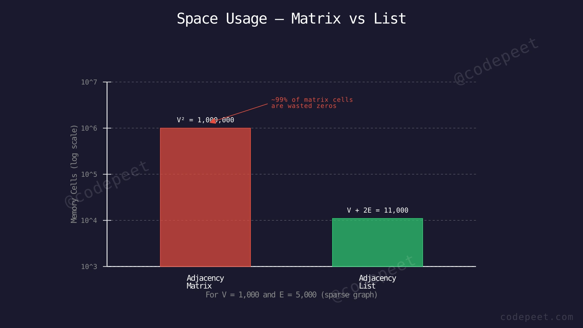
Space Complexity: O(V²)
The matrix always uses V² cells regardless of how many edges actually exist. For a graph with 1,000 vertices but only 5 edges, we still allocate 1,000,000 cells — 999,990 of which are wasted zeros. This is the key limitation of the adjacency matrix.
Why This Approach Is Not Efficient
The adjacency matrix has one critical flaw: it always uses O(V²) space, no matter how many edges the graph actually has.
Most real-world graphs are sparse — they have far fewer edges than the theoretical maximum. A social network with 1 million users does not have every user connected to every other user. Instead, each person might have a few hundred friends on average.
Consider these concrete numbers:
- V = 10,000 vertices, E = 20,000 edges (a typical sparse graph)
- Adjacency matrix space: V² = 100,000,000 cells = 100 MB (at 1 byte per cell)
- Actual edges stored: only 20,000 cells are non-zero — 99.98% of the matrix is wasted
Besides the space waste, finding all neighbors of a vertex requires scanning an entire row of V cells, even if the vertex only has 3 neighbors. This makes neighbor enumeration O(V) when it could be O(degree).
The adjacency matrix is only efficient when:
- The graph is dense (E is close to V²)
- You need O(1) edge existence checks frequently
- V is small enough that V² fits comfortably in memory
For sparse graphs (which are the majority of practical scenarios), we need a representation that stores only the edges that actually exist. This leads us to the adjacency list.
Optimal Approach - Adjacency List
Intuition
Instead of reserving space for every possible edge (V² cells), what if we only stored the edges that actually exist?
Imagine a phone contact list. You do not have a slot for every person in the world — you only store the numbers of people you actually know. Each person has their own list of contacts, and the length of each list varies.
The adjacency list works the same way. We create an array of V lists (one per vertex). For each edge (u, v):
- Add
vto vertexu's list (vertex u has neighbor v) - For undirected graphs, also add
uto vertexv's list
Now each vertex stores only its actual neighbors — no wasted space for non-existent edges.
In C++, the most idiomatic way is to use a vector of vectors: vector<vector<int>> adj(V);. Each inner vector adj[i] starts empty and grows dynamically as we add neighbors using push_back(). For weighted graphs, we use vector<vector<pair<int,int>>> adj(V); where each pair stores (neighbor, weight).
This is the standard representation used in nearly all competitive programming and real-world graph algorithms (BFS, DFS, Dijkstra, etc.) because it is both space-efficient and fast for neighbor iteration.
Step-by-Step Explanation
Let's build the adjacency list for Example 1: V = 3, edges = [(0,1), (0,2), (1,2)], undirected.
Step 1: Create 3 empty lists, one per vertex.
adj[0] = []
adj[1] = []
adj[2] = []
Step 2: Process edge (0,1). Add vertex 1 to adj[0].
adj[0] = [1]
adj[1] = []
adj[2] = []
Step 3: Since the graph is undirected, also add vertex 0 to adj[1].
adj[0] = [1]
adj[1] = [0]
adj[2] = []
Step 4: Process edge (0,2). Add vertex 2 to adj[0].
adj[0] = [1, 2]
adj[1] = [0]
adj[2] = []
Step 5: Mirror: add vertex 0 to adj[2].
adj[0] = [1, 2]
adj[1] = [0]
adj[2] = [0]
Step 6: Process edge (1,2). Add vertex 2 to adj[1].
adj[0] = [1, 2]
adj[1] = [0, 2]
adj[2] = [0]
Step 7: Mirror: add vertex 1 to adj[2].
adj[0] = [1, 2]
adj[1] = [0, 2]
adj[2] = [0, 1]
Step 8: All edges processed. The adjacency list is complete. Each vertex stores exactly the vertices it is connected to — no wasted entries.
Building an Adjacency List — Undirected Graph — Watch how each edge is added to both endpoints' neighbor lists, progressively building the complete adjacency list representation.
Algorithm
- Read the number of vertices
Vand edgesE. - Create an array of
Vempty lists (in C++:vector<vector<int>> adj(V);). - For each edge
(u, v)in the input:- Add
vtoadj[u](vertex u has neighbor v). In C++:adj[u].push_back(v); - If undirected, also add
utoadj[v]. In C++:adj[v].push_back(u); - If directed, only add to
adj[u]. - For weighted edges with weight
w, store pairs:adj[u].push_back({v, w});
- Add
- The list is now ready. To find all neighbors of vertex
i, iterate overadj[i]. - To check if edge (u, v) exists, scan
adj[u]for valuev(takes O(degree(u)) time).
Code
#include <bits/stdc++.h>
using namespace std;

int main() {
    int V, E;
    cin >> V >> E;

    // Adjacency list: V empty vectors
    vector<vector<int>> adj(V);

    for (int i = 0; i < E; i++) {
        int u, v;
        cin >> u >> v;

        adj[u].push_back(v);
        adj[v].push_back(u); // Remove for directed graph
    }

    // Print the adjacency list
    for (int i = 0; i < V; i++) {
        cout << i << " -> ";
        for (int neighbor : adj[i]) {
            cout << neighbor << " ";
        }
        cout << endl;
    }

    return 0;
}

// --- Weighted graph variant ---
// Use vector of pairs to store (neighbor, weight):
//
// vector<vector<pair<int,int>>> adj(V);
//
// for (int i = 0; i < E; i++) {
//     int u, v, w;
//     cin >> u >> v >> w;
//     adj[u].push_back({v, w});
//     adj[v].push_back({u, w}); // Remove for directed
// }
def build_adjacency_list(V, edges, directed=False):
# Create V empty lists
adj = [[] for _ in range(V)]
for u, v in edges:
adj[u].append(v)
if not directed:
adj[v].append(u) # Mirror for undirected
return adj
# Read input
V, E = map(int, input().split())
edges = []
for _ in range(E):
u, v = map(int, input().split())
edges.append((u, v))
# Build and print the list
adj = build_adjacency_list(V, edges)
for i in range(V):
print(f"{i} -> {' '.join(map(str, adj[i]))}")
# --- Weighted graph variant ---
# Store tuples (neighbor, weight):
#
# def build_weighted_list(V, edges, directed=False):
# adj = [[] for _ in range(V)]
# for u, v, w in edges:
# adj[u].append((v, w))
# if not directed:
# adj[v].append((u, w))
# return adjimport java.util.*;
public class Solution {
public static void main(String[] args) {
Scanner sc = new Scanner(System.in);
int V = sc.nextInt();
int E = sc.nextInt();
// Adjacency list: V empty ArrayLists
ArrayList<ArrayList<Integer>> adj = new ArrayList<>();
for (int i = 0; i < V; i++) {
adj.add(new ArrayList<>());
}
for (int i = 0; i < E; i++) {
int u = sc.nextInt();
int v = sc.nextInt();
adj.get(u).add(v);
adj.get(v).add(u); // Remove for directed graph
}
// Print the adjacency list
for (int i = 0; i < V; i++) {
System.out.print(i + " -> ");
for (int neighbor : adj.get(i)) {
System.out.print(neighbor + " ");
}
System.out.println();
}
}
}
// --- Weighted graph variant ---
// Use ArrayList of int[] pairs {neighbor, weight}:
//
// ArrayList<ArrayList<int[]>> adj = new ArrayList<>();
// for (int i = 0; i < V; i++) adj.add(new ArrayList<>());
//
// adj.get(u).add(new int[]{v, w});
// adj.get(v).add(new int[]{u, w}); // Remove for directedComplexity Analysis
Time Complexity:
-
Building the list: O(V + E)
- Creating V empty lists takes O(V).
- Processing each of the E edges takes O(1) per edge (appending to a vector/list is amortized O(1)).
- Total: O(V + E).
-
Checking if edge (u, v) exists: O(degree(u)) — must scan vertex u's neighbor list. In the worst case, degree(u) can be V−1, but on average for sparse graphs it is much smaller.
-
Finding all neighbors of vertex u: O(degree(u)) — just iterate over adj[u]. This is optimal because you only visit the actual neighbors, not all V vertices.
Space Complexity: O(V + E)
- V lists (one per vertex) contribute O(V).
- For an undirected graph, each edge appears in two lists, contributing 2E total entries → O(E).
- For a directed graph, each edge appears once → O(E).
- Total: O(V + E).
For sparse graphs (E << V²), this is dramatically better than the O(V²) adjacency matrix. For a graph with V = 10,000 and E = 20,000, the adjacency list uses roughly 50,000 entries vs. 100,000,000 cells for the matrix.
Summary of Trade-offs:
| Operation | Adjacency Matrix | Adjacency List |
|---|---|---|
| Space | O(V²) | O(V + E) |
| Check if edge exists | O(1) | O(degree) |
| List all neighbors | O(V) | O(degree) |
| Add an edge | O(1) | O(1) |
| Best suited for | Dense graphs, frequent edge queries | Sparse graphs, neighbor iteration |