Tree Boundary Traversal
Description
Given the root of a binary tree, return its boundary traversal in anti-clockwise order, starting from the root.
The boundary of a binary tree consists of three parts:
- Left Boundary: The nodes on the left edge of the tree, starting from the root and moving downward. At each step, prefer the left child; if it does not exist, take the right child. Exclude leaf nodes from this part.
- Leaf Nodes: All leaf nodes of the tree collected from left to right.
- Right Boundary: The nodes on the right edge of the tree, starting from the root and moving downward. At each step, prefer the right child; if it does not exist, take the left child. Exclude leaf nodes from this part. These nodes are added in reverse (bottom-up) order.
The root node is always included as the first element. Each node should appear only once in the final traversal — there must be no duplicates between the three parts.
Important edge cases:
- If the root has no left subtree, the left boundary is just the root itself.
- If the root has no right subtree, the right boundary is just the root itself.
- A single-node tree returns just the root.
Examples
Example 1
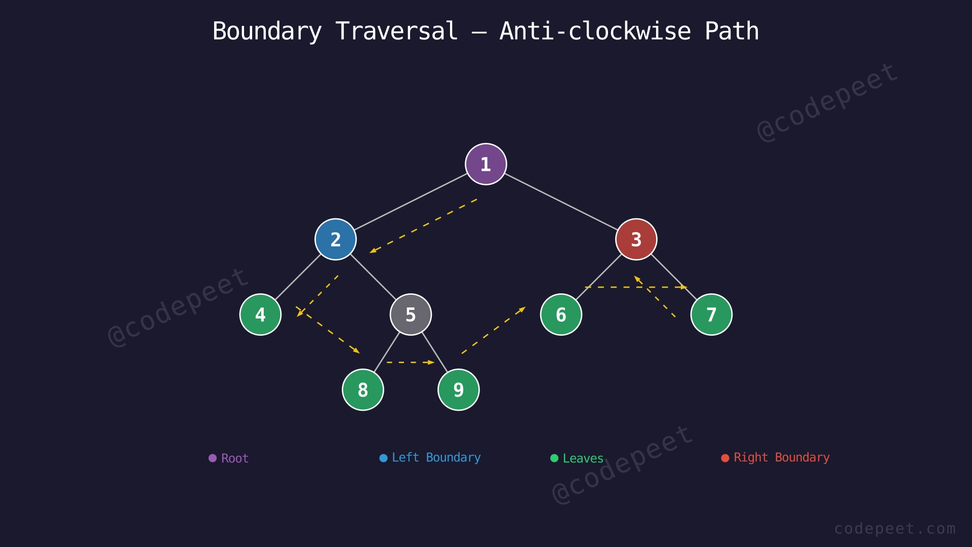
Input: root = [1, 2, 3, 4, 5, 6, 7, N, N, 8, 9, N, N, N, N]
          1
        /   \
       2     3
      / \   / \
     4   5 6   7
        / \
       8   9
Output: [1, 2, 4, 8, 9, 6, 7, 3]
Explanation:
- Left boundary (excluding leaves): Starting from root, go left → node 2. From node 2, go left → node 4 (this is a leaf, so stop). Left boundary = [1, 2].
- Leaf nodes (left to right): 4, 8, 9, 6, 7. These are all the nodes with no children, collected in the order they appear from left to right in the tree.
- Right boundary (excluding leaves, reversed): Starting from root, go right → node 3. From node 3, go right → node 7 (this is a leaf, so stop). Right boundary collected top-down = [3]. Reversed = [3].
- Combined: [1, 2] + [4, 8, 9, 6, 7] + [3] = [1, 2, 4, 8, 9, 6, 7, 3].
Example 2
Input: root = [1, N, 2, N, 3, N, 4]
  1
   \
    2
     \
      3
       \
        4
Output: [1, 4, 3, 2]
Explanation:
- Left boundary: Root has no left subtree, so the left boundary is just [1] (the root).
- Leaf nodes: Only node 4 is a leaf. Leaves = [4].
- Right boundary (excluding leaves, reversed): From root, go right → 2 (not leaf) → 3 (not leaf) → 4 (leaf, stop). Right boundary top-down = [2, 3]. Reversed = [3, 2].
- Combined: [1] + [4] + [3, 2] = [1, 4, 3, 2].
Example 3
Input: root = [1, 2, 3]
    1
   / \
  2   3
Output: [1, 2, 3]
Explanation:
- Left boundary: From root, go left → node 2 (leaf, stop). Left boundary excluding leaves = [1] (just root).
- Leaf nodes: Nodes 2 and 3 are both leaves. Leaves = [2, 3].
- Right boundary: From root, go right → node 3 (leaf, stop). Right boundary excluding leaves = []. Reversed = [].
- Combined: [1] + [2, 3] + [] = [1, 2, 3]. The root plus all leaves, since there are no non-leaf boundary nodes besides the root.
Constraints
- 1 ≤ number of nodes ≤ 10^5
- 1 ≤ node.data ≤ 10^5
Editorial
Brute Force
Intuition
The most straightforward way to find boundary nodes is to first collect complete information about the tree and then extract what we need.
Imagine taking a photograph of the entire tree — storing every node organized by its level. Once we have this complete picture, we can scan through the levels to identify which nodes are leaves, and we already know how to walk the left and right edges.
The plan is:
- BFS (level-order) traversal to store every node grouped by level
- Walk down the left edge of the tree to collect left boundary nodes (preferring left child, then right)
- Scan through our stored levels to pick out all leaf nodes from left to right
- Walk down the right edge to collect right boundary nodes, then reverse them
- Combine all three parts
Using BFS for leaf collection is overkill — we store ALL nodes just to filter out the leaves. But it works correctly and is conceptually simple: store everything, then pick what you need.
Step-by-Step Explanation
Let's trace through with the tree from Example 1:
          1
        /   \
       2     3
      / \   / \
     4   5 6   7
        / \
       8   9
Phase 1: BFS to store all levels
Step 1: Initialize queue with root (1). Start BFS.
Step 2: Process level 0: Dequeue node 1. Enqueue children 2, 3. Level 0 = [1].
Step 3: Process level 1: Dequeue node 2 (enqueue 4, 5), dequeue node 3 (enqueue 6, 7). Level 1 = [2, 3].
Step 4: Process level 2: Dequeue nodes 4 (no children), 5 (enqueue 8, 9), 6 (no children), 7 (no children). Level 2 = [4, 5, 6, 7].
Step 5: Process level 3: Dequeue nodes 8, 9 (both no children). Level 3 = [8, 9]. Queue empty.
All levels stored: [[1], [2, 3], [4, 5, 6, 7], [8, 9]]
Phase 2: Extract boundary parts
Step 6: Root goes first: result = [1].
Step 7: Left boundary: Walk from root.left (2). Node 2 is not a leaf → add. Move to 2.left = 4, which IS a leaf → stop. Left boundary (excluding root and leaves) = [2]. Result = [1, 2].
Step 8: Leaves from stored levels: Scan each level and pick nodes with no children. Level 0: 1 has children, skip. Level 1: 2 has children, 3 has children, skip both. Level 2: 4 is leaf ✓, 5 has children (skip), 6 is leaf ✓, 7 is leaf ✓. Level 3: 8 is leaf ✓, 9 is leaf ✓. Leaves = [4, 8, 9, 6, 7].
Wait — the level-by-level scan gives leaves in level order: [4, 6, 7, 8, 9]. But we need them in left-to-right order which is [4, 8, 9, 6, 7]. Since BFS visits nodes left-to-right within each level, the leaves from the stored levels are already in the correct left-to-right reading order: level 2 gives [4, 6, 7] and level 3 gives [8, 9]. But in actual left-to-right tree order, 8 and 9 come before 6 and 7 because they are children of 5 which is between 4 and 6.
This is actually a problem with the BFS approach! BFS gives leaves in level-order (breadth-first) rather than true left-to-right order. For this specific tree, the BFS leaf order is [4, 6, 7, 8, 9] but the correct order is [4, 8, 9, 6, 7].
To fix this, we must collect leaves using DFS (depth-first, going left before right), NOT from the BFS levels. So the corrected approach uses BFS only for storage, but collects leaves via a separate DFS pass.
Result after collecting leaves via DFS: [1, 2, 4, 8, 9, 6, 7].
Step 9: Right boundary: Walk from root.right (3). Node 3 is not a leaf → collect. Move to 3.right = 7, which IS a leaf → stop. Right boundary (top-down) = [3]. Reversed = [3]. Result = [1, 2, 4, 8, 9, 6, 7, 3].
Final result: [1, 2, 4, 8, 9, 6, 7, 3].
Brute Force — BFS Level Collection + Boundary Extraction — Watch how BFS visits all nodes level by level, storing them for later boundary extraction. After BFS completes, we walk left/right edges and collect leaves.
Algorithm
- Perform BFS (level-order traversal) to store all nodes grouped by level
- Add the root to the result
- If root is a leaf, return [root]
- Left boundary: Starting from root.left, walk downward preferring left child (if null, take right). Add each non-leaf node to result. Stop when reaching a leaf.
- Leaf nodes: Perform a DFS traversal of the entire tree. Add every leaf node (no children) to the result in left-to-right order.
- Right boundary: Starting from root.right, walk downward preferring right child (if null, take left). Collect each non-leaf node. Reverse the collected nodes and add to result.
- Return the combined result
Code
#include <vector>
#include <queue>
using namespace std;

class Solution {
public:
    bool isLeaf(Node* node) {
        return !node->left && !node->right;
    }

    void dfsLeaves(Node* node, vector<int>& res) {
        if (!node) return;
        if (isLeaf(node)) {
            res.push_back(node->data);
            return;
        }
        dfsLeaves(node->left, res);
        dfsLeaves(node->right, res);
    }

    vector<int> boundaryTraversal(Node* root) {
        if (!root) return {};

        vector<int> result;
        result.push_back(root->data);
        if (isLeaf(root)) return result;

        // Step 1: BFS to store all nodes by level
        vector<vector<Node*>> levels;
        queue<Node*> q;
        q.push(root);
        while (!q.empty()) {
            int sz = q.size();
            vector<Node*> level;
            for (int i = 0; i < sz; i++) {
                Node* curr = q.front();
                q.pop();
                level.push_back(curr);
                if (curr->left) q.push(curr->left);
                if (curr->right) q.push(curr->right);
            }
            levels.push_back(level);
        }

        // Step 2: Left boundary (walk left edge, exclude leaves)
        Node* node = root->left;
        while (node && !isLeaf(node)) {
            result.push_back(node->data);
            node = node->left ? node->left : node->right;
        }

        // Step 3: Leaf nodes via DFS (not from BFS levels)
        dfsLeaves(root, result);

        // Step 4: Right boundary (walk right edge, reversed)
        vector<int> rightBound;
        node = root->right;
        while (node && !isLeaf(node)) {
            rightBound.push_back(node->data);
            node = node->right ? node->right : node->left;
        }
        for (int i = rightBound.size() - 1; i >= 0; i--) {
            result.push_back(rightBound[i]);
        }

        return result;
    }
};
from collections import deque
class Solution:
def boundaryTraversal(self, root):
if not root:
return []
def is_leaf(node):
return not node.left and not node.right
def dfs_leaves(node, res):
if not node:
return
if is_leaf(node):
res.append(node.data)
return
dfs_leaves(node.left, res)
dfs_leaves(node.right, res)
result = [root.data]
if is_leaf(root):
return result
# Step 1: BFS to store all nodes by level
levels = []
queue = deque([root])
while queue:
level = []
for _ in range(len(queue)):
curr = queue.popleft()
level.append(curr)
if curr.left:
queue.append(curr.left)
if curr.right:
queue.append(curr.right)
levels.append(level)
# Step 2: Left boundary (walk left edge, exclude leaves)
node = root.left
while node and not is_leaf(node):
result.append(node.data)
node = node.left if node.left else node.right
# Step 3: Leaf nodes via DFS
dfs_leaves(root, result)
# Step 4: Right boundary (reversed)
right_bound = []
node = root.right
while node and not is_leaf(node):
right_bound.append(node.data)
node = node.right if node.right else node.left
result.extend(reversed(right_bound))
return resultimport java.util.*;
class Solution {
boolean isLeaf(Node node) {
return node.left == null && node.right == null;
}
void dfsLeaves(Node node, ArrayList<Integer> res) {
if (node == null) return;
if (isLeaf(node)) {
res.add(node.data);
return;
}
dfsLeaves(node.left, res);
dfsLeaves(node.right, res);
}
ArrayList<Integer> boundaryTraversal(Node root) {
ArrayList<Integer> result = new ArrayList<>();
if (root == null) return result;
result.add(root.data);
if (isLeaf(root)) return result;
// Step 1: BFS to store all nodes by level
List<List<Node>> levels = new ArrayList<>();
Queue<Node> queue = new LinkedList<>();
queue.add(root);
while (!queue.isEmpty()) {
int size = queue.size();
List<Node> level = new ArrayList<>();
for (int i = 0; i < size; i++) {
Node curr = queue.poll();
level.add(curr);
if (curr.left != null) queue.add(curr.left);
if (curr.right != null) queue.add(curr.right);
}
levels.add(level);
}
// Step 2: Left boundary (exclude leaves)
Node node = root.left;
while (node != null && !isLeaf(node)) {
result.add(node.data);
node = node.left != null ? node.left : node.right;
}
// Step 3: Leaf nodes via DFS
dfsLeaves(root, result);
// Step 4: Right boundary (reversed)
List<Integer> rightBound = new ArrayList<>();
node = root.right;
while (node != null && !isLeaf(node)) {
rightBound.add(node.data);
node = node.right != null ? node.right : node.left;
}
Collections.reverse(rightBound);
result.addAll(rightBound);
return result;
}
}Complexity Analysis
Time Complexity: O(n)
The BFS traversal visits all n nodes once: O(n). The left boundary walk visits at most h nodes: O(h). The DFS for leaves visits all n nodes once: O(n). The right boundary walk visits at most h nodes: O(h). Total: O(n) + O(h) + O(n) + O(h) = O(n), since h ≤ n.
Space Complexity: O(n)
The BFS level storage holds all n nodes organized by level. The queue during BFS holds at most the width of the tree (up to n/2 nodes for a complete tree). The DFS recursion stack uses O(h) space. The right boundary storage uses O(h). The dominant factor is the BFS level storage: O(n).
Why This Approach Is Not Efficient
The brute force approach stores all n nodes in level arrays during BFS, but we only ever use a small fraction of them. For a tree with n = 10^5 nodes, we allocate memory for 10^5 node references just to later discard most of them.
The BFS level storage is fundamentally wasteful because:
- Left boundary needs at most h nodes (one per level, following the leftmost path)
- Leaves can be collected directly during any traversal without pre-storing all nodes
- Right boundary needs at most h nodes (one per level, following the rightmost path)
For a balanced tree with n = 10^5, the height h ≈ 17. The BFS approach stores all 10^5 nodes, but we only need O(h) ≈ 17 nodes for the boundary edges. The leaf collection doesn't benefit from level storage either — a simple DFS does it with O(h) stack space instead of O(n) stored nodes.
The key insight is that each of the three boundary parts can be collected independently and directly — we don't need the global picture that BFS provides. The left boundary is just a walk down the left edge. The leaves are found by any DFS. The right boundary is a walk down the right edge. None of these require knowing all nodes at all levels.
Optimal Approach - Three-Part Recursive Decomposition
Intuition
Instead of collecting all nodes and then filtering, we decompose the boundary traversal into three independent, focused sub-tasks — each with clean, simple logic:
Part 1 — Left Boundary (top-down): Starting from the root's left child, walk downward. At each node, prefer the left child; if it doesn't exist, take the right child. Stop when you reach a leaf. Add each non-leaf node to the result as you go down.
Part 2 — Leaf Nodes (left-to-right): Do a standard depth-first traversal of the entire tree (go left first, then right). Whenever you encounter a node with no children, add it to the result. This naturally gives leaves in left-to-right order.
Part 3 — Right Boundary (bottom-up): Starting from the root's right child, walk downward. At each node, prefer the right child; if it doesn't exist, take the left child. Stop when you reach a leaf. But here's the trick — we need these nodes in reverse (bottom-up) order. We can either collect them top-down and reverse, or use recursion to add them after the recursive call returns (post-order style).
These three parts are completely independent. Each can be implemented as a small, focused helper function. No node is processed by more than two parts (leaf nodes are only collected in Part 2, not in Parts 1 or 3), ensuring no duplicates.
The beauty of this approach is its modularity — if any part has a bug, you can test and fix it in isolation.
Step-by-Step Explanation
Let's trace through with the tree from Example 1:
          1
        /   \
       2     3
      / \   / \
     4   5 6   7
        / \
       8   9
Step 1: Add root (1) to result. Result = [1]. The root is always the first element.
Part 1: Left Boundary
Step 2: Start at root.left = node 2. Is it a leaf? No (has children 4, 5). Add 2 to result. Result = [1, 2].
Step 3: Prefer left child: 2.left = node 4. Is it a leaf? Yes (no children). Stop — leaves are collected separately. Left boundary collection is done.
Part 2: Leaf Nodes (DFS left-to-right)
Step 4: DFS from root. Go left to node 2, then left to node 4. Node 4 is a leaf — add it. Result = [1, 2, 4].
Step 5: Backtrack to node 2, go right to node 5. Node 5 has children, not a leaf. Go left to node 8. Node 8 is a leaf — add it. Result = [1, 2, 4, 8].
Step 6: Backtrack to node 5, go right to node 9. Node 9 is a leaf — add it. Result = [1, 2, 4, 8, 9].
Step 7: Backtrack to root, go right to node 3. Go left to node 6. Node 6 is a leaf — add it. Result = [1, 2, 4, 8, 9, 6].
Step 8: Backtrack to node 3, go right to node 7. Node 7 is a leaf — add it. Result = [1, 2, 4, 8, 9, 6, 7].
Part 3: Right Boundary (bottom-up using post-order recursion)
Step 9: Start at root.right = node 3. Is it a leaf? No (has children 6, 7). Prefer right child: 3.right = node 7. Is it a leaf? Yes — stop recursion.
Step 10: Returning from recursion at node 3 — add 3 to result (post-order gives bottom-up order). Result = [1, 2, 4, 8, 9, 6, 7, 3].
Final Result: [1, 2, 4, 8, 9, 6, 7, 3].
Three-Part Decomposition — Left Boundary, Leaves, Right Boundary — Watch the three independent phases: first the left boundary is walked top-down (blue), then leaves are collected left-to-right via DFS (green), finally the right boundary is collected bottom-up (red).
Algorithm
- Add the root to the result. If root is a leaf, return [root]
- collectLeftBoundary(root.left):
- If node is null or a leaf, return
- Add node's value to result
- If node has a left child, recurse on left child
- Otherwise, recurse on right child
- collectLeaves(root):
- If node is null, return
- If node is a leaf, add its value to result
- Recurse on left child, then right child
- collectRightBoundary(root.right):
- If node is null or a leaf, return
- If node has a right child, recurse on right child
- Otherwise, recurse on left child
- After the recursive call, add node's value to result (post-order = reverse order)
- Return the combined result
Code
#include <vector>
using namespace std;

class Solution {
public:
    bool isLeaf(Node* node) {
        return !node->left && !node->right;
    }

    // Collect left boundary nodes (top-down, exclude leaves)
    void collectLeft(Node* node, vector<int>& res) {
        if (!node || isLeaf(node)) return;
        res.push_back(node->data);
        if (node->left)
            collectLeft(node->left, res);
        else
            collectLeft(node->right, res);
    }

    // Collect all leaf nodes (left to right via DFS)
    void collectLeaves(Node* node, vector<int>& res) {
        if (!node) return;
        if (isLeaf(node)) {
            res.push_back(node->data);
            return;
        }
        collectLeaves(node->left, res);
        collectLeaves(node->right, res);
    }

    // Collect right boundary nodes (bottom-up via post-order)
    void collectRight(Node* node, vector<int>& res) {
        if (!node || isLeaf(node)) return;
        if (node->right)
            collectRight(node->right, res);
        else
            collectRight(node->left, res);
        res.push_back(node->data);  // add AFTER recursion = reverse
    }

    vector<int> boundaryTraversal(Node* root) {
        if (!root) return {};

        vector<int> result;
        result.push_back(root->data);

        if (isLeaf(root)) return result;

        collectLeft(root->left, result);
        collectLeaves(root, result);
        collectRight(root->right, result);

        return result;
    }
};
class Solution:
def boundaryTraversal(self, root):
if not root:
return []
def is_leaf(node):
return not node.left and not node.right
def collect_left(node):
"""Collect left boundary top-down, exclude leaves."""
if not node or is_leaf(node):
return
result.append(node.data)
if node.left:
collect_left(node.left)
else:
collect_left(node.right)
def collect_leaves(node):
"""Collect all leaves left-to-right via DFS."""
if not node:
return
if is_leaf(node):
result.append(node.data)
return
collect_leaves(node.left)
collect_leaves(node.right)
def collect_right(node):
"""Collect right boundary bottom-up via post-order."""
if not node or is_leaf(node):
return
if node.right:
collect_right(node.right)
else:
collect_right(node.left)
result.append(node.data) # add AFTER recursion = reverse
result = [root.data]
if is_leaf(root):
return result
collect_left(root.left)
collect_leaves(root)
collect_right(root.right)
return resultimport java.util.ArrayList;
class Solution {
boolean isLeaf(Node node) {
return node.left == null && node.right == null;
}
// Collect left boundary top-down, exclude leaves
void collectLeft(Node node, ArrayList<Integer> res) {
if (node == null || isLeaf(node)) return;
res.add(node.data);
if (node.left != null)
collectLeft(node.left, res);
else
collectLeft(node.right, res);
}
// Collect all leaves left-to-right via DFS
void collectLeaves(Node node, ArrayList<Integer> res) {
if (node == null) return;
if (isLeaf(node)) {
res.add(node.data);
return;
}
collectLeaves(node.left, res);
collectLeaves(node.right, res);
}
// Collect right boundary bottom-up via post-order
void collectRight(Node node, ArrayList<Integer> res) {
if (node == null || isLeaf(node)) return;
if (node.right != null)
collectRight(node.right, res);
else
collectRight(node.left, res);
res.add(node.data); // add AFTER recursion = reverse
}
ArrayList<Integer> boundaryTraversal(Node root) {
ArrayList<Integer> result = new ArrayList<>();
if (root == null) return result;
result.add(root.data);
if (isLeaf(root)) return result;
collectLeft(root.left, result);
collectLeaves(root, result);
collectRight(root.right, result);
return result;
}
}Complexity Analysis
Time Complexity: O(n)
Each node in the tree is visited at most twice — once during the left/right boundary walk (which only visits O(h) nodes along one edge), and once during the DFS leaf collection (which visits all n nodes). Since h ≤ n, the total work is O(n) + O(h) = O(n).
More precisely:
- Left boundary walk: O(h) — follows one path from root downward
- Leaf DFS: O(n) — visits every node once to check if it's a leaf
- Right boundary walk: O(h) — follows one path from root downward
- Total: O(h) + O(n) + O(h) = O(n)
Space Complexity: O(h)
The main space usage is the recursion stack. The deepest recursion occurs during the leaf collection DFS, which can go h levels deep. The left and right boundary walks each use O(h) recursion depth. No additional data structures (like level arrays) are needed beyond the result list.
For a balanced binary tree, h = O(log n), so the space is O(log n). For a skewed tree, h = O(n), so the space is O(n) in the worst case. This is a significant improvement over the brute force's unconditional O(n) space for level storage.