Prim's Algorithm
Description
Given a weighted, undirected, and connected graph with V vertices (numbered 0 to V-1) and E edges, find the sum of the weights of the edges in the Minimum Spanning Tree (MST) of the graph using Prim's algorithm.
Prim's algorithm builds the MST by growing it one vertex at a time. Starting from an arbitrary vertex, the algorithm repeatedly picks the cheapest edge that connects a vertex already in the MST to a vertex not yet in the MST. This process continues until all vertices are included.
The graph is provided as a list of edges, where each edge is represented as [u, v, w], indicating an undirected edge between vertex u and vertex v with weight w.
Examples
Example 1
Input: V = 3, E = 3, edges = [[0, 1, 5], [1, 2, 3], [0, 2, 1]]
Output: 4
Explanation: Starting Prim's from vertex 0:
- Vertex 0 is added to MST. Edges from MST: 0-1 (w=5), 0-2 (w=1). Minimum: 0-2 (w=1). Add vertex 2.
- MST = {0, 2}. Edges from MST to non-MST: 0-1 (w=5), 2-1 (w=3). Minimum: 2-1 (w=3). Add vertex 1.
- All vertices in MST. Total weight = 1 + 3 = 4.
Example 2
Input: V = 2, E = 1, edges = [[0, 1, 5]]
Output: 5
Explanation: Only one edge exists. Starting from vertex 0, the only edge to a non-MST vertex is 0-1 (weight 5). Add it. MST weight = 5.
Example 3
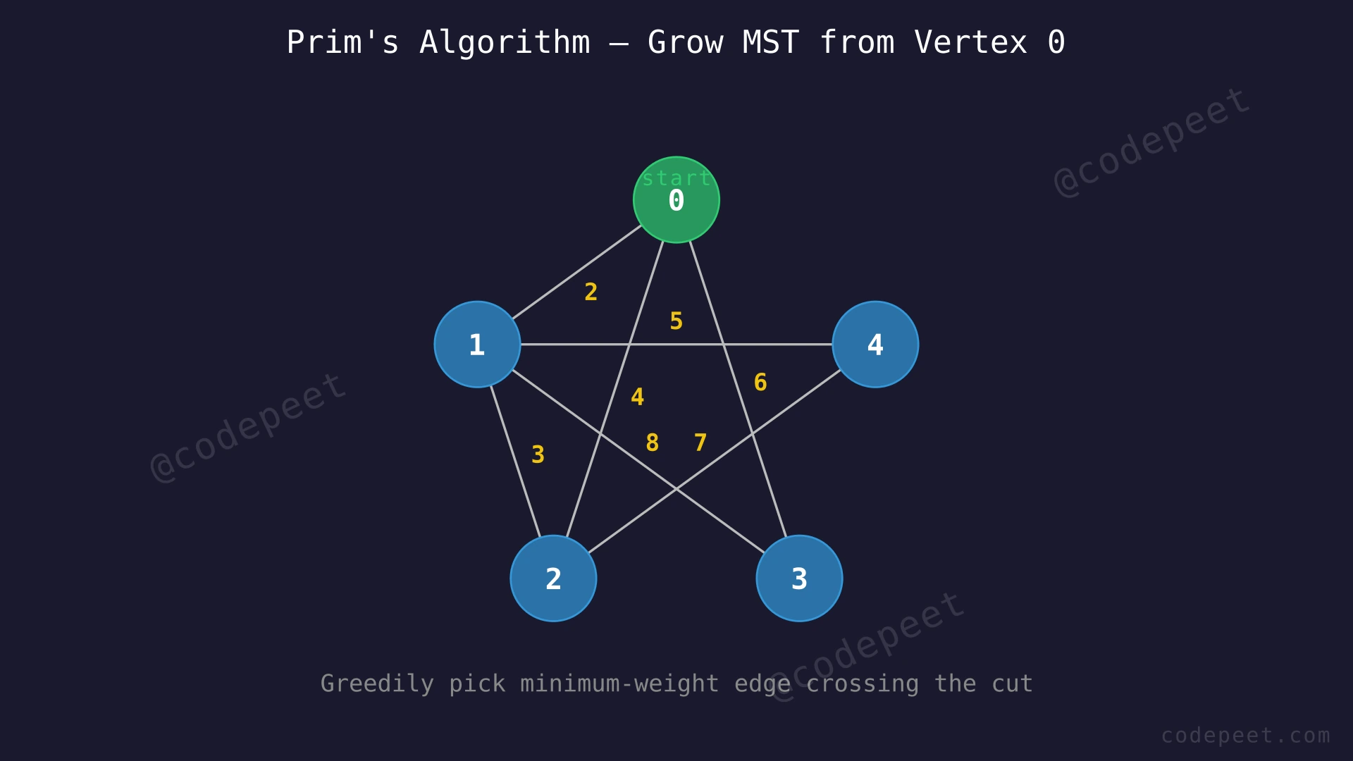
Input: V = 5, E = 7, edges = [[0,1,2], [1,2,3], [0,2,4], [1,4,5], [0,3,6], [2,4,7], [1,3,8]]
Output: 16
Explanation: Starting from vertex 0, Prim's algorithm adds edges in this order: 0-1 (w=2), 1-2 (w=3), 1-4 (w=5), 0-3 (w=6). Total weight = 2 + 3 + 5 + 6 = 16. Note that edge 0-2 (w=4) is skipped because vertex 2 is already in the MST when its turn comes (reached earlier via the cheaper path 0→1→2 with edge weight 3).
Constraints
- 2 ≤ V ≤ 1000
- V-1 ≤ E ≤ V × (V-1) / 2
- 1 ≤ w ≤ 1000
- The graph is connected
- No self-loops or multiple edges between the same pair of vertices
Editorial
Brute Force
Intuition
Prim's algorithm grows the MST from a starting vertex by always picking the cheapest edge that connects a vertex inside the MST to one outside it. The simplest way to implement this is to maintain a key array where key[v] stores the minimum weight edge that can connect vertex v to the current MST.
At each step, we need to find the unvisited vertex with the smallest key value. The most straightforward way to do this is a linear scan through all V vertices, checking each one. After picking the minimum, we add it to the MST and update the key values of its neighbors.
Think of building a train network between cities. You start at one city (vertex 0) and look at all the rail lines you could build from there. You pick the cheapest one and build it. Now from both connected cities, you look at all possible rail lines to unconnected cities, pick the cheapest, and build it. At each step, to find the cheapest rail line, you check every unconnected city — a slow but reliable approach.
Step-by-Step Explanation
Let's trace through with V = 5, E = 7, edges = [[0,1,2], [1,2,3], [0,2,4], [1,4,5], [0,3,6], [2,4,7], [1,3,8]]:
Step 1: Initialize
key = [0, INF, INF, INF, INF], inMST = [F, F, F, F, F]
Vertex 0 gets key 0 so it is picked first.
Step 2: Linear scan — find minimum key among non-MST vertices
Scan v=0 (key=0), v=1 (key=INF), v=2 (key=INF), v=3 (key=INF), v=4 (key=INF)
Minimum: vertex 0 (key=0). Mark inMST[0] = true. MST weight += 0 = 0.
Step 3: Update keys from vertex 0's neighbors
Edge 0-1 (w=2): key[1] = min(INF, 2) = 2. Updated.
Edge 0-2 (w=4): key[2] = min(INF, 4) = 4. Updated.
Edge 0-3 (w=6): key[3] = min(INF, 6) = 6. Updated.
key = [0, 2, 4, 6, INF]
Step 4: Linear scan — find minimum key
Scan v=1 (key=2), v=2 (key=4), v=3 (key=6), v=4 (key=INF)
Minimum: vertex 1 (key=2). Mark inMST[1] = true. MST weight += 2 = 2.
Step 5: Update keys from vertex 1's neighbors
Edge 1-0 (visited, skip)
Edge 1-2 (w=3): key[2] = min(4, 3) = 3. Updated! Better path found.
Edge 1-3 (w=8): key[3] = min(6, 8) = 6. No change (0-3 is cheaper).
Edge 1-4 (w=5): key[4] = min(INF, 5) = 5. Updated.
key = [0, 2, 3, 6, 5]
Step 6: Linear scan — find minimum key
Scan v=2 (key=3), v=3 (key=6), v=4 (key=5)
Minimum: vertex 2 (key=3). Mark inMST[2] = true. MST weight += 3 = 5.
Step 7: Update keys from vertex 2's neighbors
Edge 2-0 (visited), Edge 2-1 (visited)
Edge 2-4 (w=7): key[4] = min(5, 7) = 5. No change (1-4 is cheaper).
key = [0, 2, 3, 6, 5]
Step 8: Linear scan — find minimum key
Scan v=3 (key=6), v=4 (key=5)
Minimum: vertex 4 (key=5). Mark inMST[4] = true. MST weight += 5 = 10.
Step 9: Update keys from vertex 4's neighbors
All neighbors (1, 2) already visited. No updates.
Step 10: Linear scan — only vertex 3 remains
Vertex 3 (key=6). Mark inMST[3] = true. MST weight += 6 = 16.
Result: MST weight = 16.
Prim's Algorithm — Linear Scan for Minimum Key — Watch how Prim's algorithm grows the MST from vertex 0, picking the cheapest connecting edge at each step by scanning all vertices linearly.
Algorithm
- Build an adjacency list from the edge list
- Create a key array of size V, initialized to INF. Set key[0] = 0 (starting vertex)
- Create a boolean array inMST of size V, initialized to false
- Initialize mst_weight = 0
- Repeat V times:
a. Linear scan all V vertices to find the non-MST vertex u with minimum key[u]
b. Mark inMST[u] = true, add key[u] to mst_weight
c. For each neighbor v of u with edge weight w:- If v is not in MST and w < key[v], update key[v] = w
- Return mst_weight
Code
#include <vector>
#include <climits>
using namespace std;

class Solution {
public:
    int spanningTree(int V, int E,
                     vector<vector<int>>& edges) {
        vector<vector<pair<int,int>>> adj(V);
        for (auto& e : edges) {
            adj[e[0]].push_back({e[1], e[2]});
            adj[e[1]].push_back({e[0], e[2]});
        }

        vector<int> key(V, INT_MAX);
        vector<bool> inMST(V, false);
        key[0] = 0;
        int mstWeight = 0;

        for (int i = 0; i < V; i++) {
            // Linear scan for minimum key
            int u = -1;
            for (int v = 0; v < V; v++) {
                if (!inMST[v] &&
                    (u == -1 || key[v] < key[u]))
                    u = v;
            }

            inMST[u] = true;
            mstWeight += key[u];

            // Update keys of neighbors
            for (auto& [v, w] : adj[u]) {
                if (!inMST[v] && w < key[v])
                    key[v] = w;
            }
        }

        return mstWeight;
    }
};
class Solution:
def spanningTree(self, V, E, edges):
adj = [[] for _ in range(V)]
for u, v, w in edges:
adj[u].append((v, w))
adj[v].append((u, w))
key = [float('inf')] * V
in_mst = [False] * V
key[0] = 0
mst_weight = 0
for _ in range(V):
# Linear scan for minimum key vertex
u = -1
for v in range(V):
if not in_mst[v] and \
(u == -1 or key[v] < key[u]):
u = v
in_mst[u] = True
mst_weight += key[u]
# Update keys of adjacent vertices
for v, w in adj[u]:
if not in_mst[v] and w < key[v]:
key[v] = w
return mst_weightimport java.util.*;
class Solution {
int spanningTree(int V, int E,
int[][] edges) {
List<int[]>[] adj = new ArrayList[V];
for (int i = 0; i < V; i++)
adj[i] = new ArrayList<>();
for (int[] e : edges) {
adj[e[0]].add(new int[]{e[1], e[2]});
adj[e[1]].add(new int[]{e[0], e[2]});
}
int[] key = new int[V];
boolean[] inMST = new boolean[V];
Arrays.fill(key, Integer.MAX_VALUE);
key[0] = 0;
int mstWeight = 0;
for (int i = 0; i < V; i++) {
// Linear scan for minimum key
int u = -1;
for (int v = 0; v < V; v++) {
if (!inMST[v] &&
(u == -1 || key[v] < key[u]))
u = v;
}
inMST[u] = true;
mstWeight += key[u];
for (int[] pair : adj[u]) {
int v = pair[0], w = pair[1];
if (!inMST[v] && w < key[v])
key[v] = w;
}
}
return mstWeight;
}
}Complexity Analysis
Time Complexity: O(V^2)
The outer loop runs V times. In each iteration, the linear scan to find the minimum key vertex takes O(V) time. The key update step iterates over the neighbors of the chosen vertex, and across all iterations, this totals O(E) since each edge is examined at most twice (once from each endpoint). So the total time is O(V × V + E) = O(V^2 + E). Since E ≤ V^2, this simplifies to O(V^2).
Space Complexity: O(V + E)
We need O(V) for the key array and the inMST boolean array, plus O(E) for the adjacency list representation of the graph.
Why This Approach Is Not Efficient
The O(V^2) approach spends most of its time on the linear scan to find the minimum key vertex. In each of V iterations, we scan all V vertices — even if only a handful of vertices had their keys updated since the last scan.
For sparse graphs where E is much smaller than V^2 (for example, E ≈ V), this is wasteful. If V = 1000 and E = 2000, the linear scan alone takes V^2 = 10^6 operations, but only about 2000 key updates ever happen. We are doing far more comparison work than necessary.
The key insight: the "find the minimum" operation is exactly what a min-heap (priority queue) is designed for. A min-heap can:
- Extract the minimum element in O(log V) time
- Insert or decrease a key in O(log V) time
By replacing the linear scan with a priority queue, each of the V extract-min operations costs O(log V) instead of O(V), and each of the E key updates costs O(log V) instead of O(1). The total becomes O((V + E) × log V), which for sparse graphs is significantly better than O(V^2).
Important nuance: For dense graphs where E ≈ V^2, the O(V^2) approach is actually competitive with or even better than the priority queue approach O(V^2 log V). The linear scan version is preferred when the graph is dense (stored as an adjacency matrix). The priority queue version wins on sparse graphs.
Optimal Approach - Prim's with Priority Queue
Intuition
The core idea of Prim's algorithm stays the same: grow the MST one vertex at a time, always picking the cheapest edge connecting the MST to a non-MST vertex. The improvement is in how we find that cheapest edge.
Instead of scanning all vertices each time, we use a min-heap (priority queue) that always keeps the cheapest available edges at the top. When we add a vertex to the MST, we push all its edges to unvisited neighbors into the heap. The heap automatically sorts them, so the next cheapest edge is always at the top — ready to extract in O(log V) time.
Imagine you are shopping at a market with hundreds of stalls. The linear scan approach is like walking past every stall each time you want to buy the cheapest item. The priority queue approach is like having an assistant who maintains a sorted shortlist of the best deals — you just ask for the top deal each time, and the assistant updates the list whenever new stalls open up.
One subtlety: since we push edges without removing stale ones, the heap may contain outdated entries (edges to vertices already in the MST). We handle this by simply skipping any extracted vertex that is already visited. This is called the lazy deletion strategy — it is simpler to code and performs well in practice.
Step-by-Step Explanation
Let's trace through with V = 5, E = 7, edges = [[0,1,2], [1,2,3], [0,2,4], [1,4,5], [0,3,6], [2,4,7], [1,3,8]]:
Step 1: Initialize
Push (weight=0, vertex=0) into min-heap. visited = [F, F, F, F, F]. MST weight = 0.
Step 2: Extract min from heap → (0, vertex 0)
Mark vertex 0 as visited. MST weight += 0 = 0.
Push edges from vertex 0: (2, v=1), (4, v=2), (6, v=3).
Heap: [(2,1), (4,2), (6,3)]
Step 3: Extract min → (2, vertex 1)
Vertex 1 not visited → mark visited. MST weight += 2 = 2.
Push edges from vertex 1 to unvisited: (3, v=2), (5, v=4), (8, v=3).
Heap: [(3,2), (4,2), (5,4), (6,3), (8,3)]
Step 4: Extract min → (3, vertex 2)
Vertex 2 not visited → mark visited. MST weight += 3 = 5.
Push edges from vertex 2 to unvisited: (7, v=4).
Heap: [(4,2), (5,4), (6,3), (7,4), (8,3)]
Step 5: Extract min → (4, vertex 2)
Vertex 2 is ALREADY visited → skip this stale entry.
Heap: [(5,4), (6,3), (7,4), (8,3)]
Step 6: Extract min → (5, vertex 4)
Vertex 4 not visited → mark visited. MST weight += 5 = 10.
Vertex 4's neighbors (1, 2) are all visited. No new pushes.
Heap: [(6,3), (7,4), (8,3)]
Step 7: Extract min → (6, vertex 3)
Vertex 3 not visited → mark visited. MST weight += 6 = 16.
All vertices now visited. MST complete.
Result: MST weight = 16.
Prim's Algorithm — Priority Queue Optimization — Watch how the priority queue always provides the cheapest edge in O(log V) time, and how stale entries are lazily discarded when extracted.
Algorithm
- Build an adjacency list from the edge list
- Create a min-heap (priority queue) and push (weight=0, vertex=0)
- Create a boolean array visited of size V, initialized to false
- Initialize mst_weight = 0
- While the priority queue is not empty:
a. Extract the minimum (weight, vertex) from the heap → O(log V)
b. If vertex is already visited, skip it (stale entry)
c. Mark vertex as visited, add weight to mst_weight
d. For each edge (vertex → neighbor, edge_weight):- If neighbor is not visited, push (edge_weight, neighbor) into the heap → O(log V)
- Return mst_weight
Code
#include <vector>
#include <queue>
using namespace std;

class Solution {
public:
    int spanningTree(int V, int E,
                     vector<vector<int>>& edges) {
        vector<vector<pair<int,int>>> adj(V);
        for (auto& e : edges) {
            adj[e[0]].push_back({e[1], e[2]});
            adj[e[1]].push_back({e[0], e[2]});
        }

        // Min-heap: {weight, vertex}
        priority_queue<pair<int,int>,
                       vector<pair<int,int>>,
                       greater<pair<int,int>>> pq;

        vector<bool> visited(V, false);
        pq.push({0, 0});
        int mstWeight = 0;

        while (!pq.empty()) {
            auto [w, u] = pq.top();
            pq.pop();

            // Skip stale entries
            if (visited[u]) continue;

            visited[u] = true;
            mstWeight += w;

            for (auto& [v, edgeW] : adj[u]) {
                if (!visited[v])
                    pq.push({edgeW, v});
            }
        }

        return mstWeight;
    }
};
import heapq
class Solution:
def spanningTree(self, V, E, edges):
adj = [[] for _ in range(V)]
for u, v, w in edges:
adj[u].append((w, v))
adj[v].append((w, u))
visited = [False] * V
pq = [(0, 0)] # (weight, vertex)
mst_weight = 0
while pq:
w, u = heapq.heappop(pq)
# Skip stale entries
if visited[u]:
continue
visited[u] = True
mst_weight += w
for edge_w, v in adj[u]:
if not visited[v]:
heapq.heappush(pq, (edge_w, v))
return mst_weightimport java.util.*;
class Solution {
int spanningTree(int V, int E,
int[][] edges) {
List<int[]>[] adj = new ArrayList[V];
for (int i = 0; i < V; i++)
adj[i] = new ArrayList<>();
for (int[] e : edges) {
adj[e[0]].add(new int[]{e[1], e[2]});
adj[e[1]].add(new int[]{e[0], e[2]});
}
// Min-heap: {weight, vertex}
PriorityQueue<int[]> pq =
new PriorityQueue<>(
(a, b) -> a[0] - b[0]);
boolean[] visited = new boolean[V];
pq.offer(new int[]{0, 0});
int mstWeight = 0;
while (!pq.isEmpty()) {
int[] top = pq.poll();
int w = top[0], u = top[1];
// Skip stale entries
if (visited[u]) continue;
visited[u] = true;
mstWeight += w;
for (int[] pair : adj[u]) {
if (!visited[pair[0]])
pq.offer(
new int[]{pair[1], pair[0]});
}
}
return mstWeight;
}
}Complexity Analysis
Time Complexity: O((E + V) × log V)
Each vertex is extracted from the priority queue exactly once, and each edge causes at most one insertion into the queue. The total number of heap operations is at most V extractions + E insertions. Each heap operation (insert or extract-min) takes O(log V) time since the heap contains at most V elements at any time (in the worst case, up to E elements with lazy deletion, but log E = O(log V) since E ≤ V^2). So the total time is O((V + E) × log V).
For sparse graphs (E ≈ V), this is O(V log V) — much better than the O(V^2) linear scan.
For dense graphs (E ≈ V^2), this is O(V^2 log V) — slightly worse than O(V^2). In that case, prefer the linear scan version.
Space Complexity: O(V + E)
We need O(V) for the visited array, O(E) for the adjacency list, and the priority queue can hold up to O(E) elements in the worst case (with lazy deletion). The total is O(V + E).