Quick Sort
Description
Given an array of integers, sort the array in ascending order using the Quick Sort algorithm.
Quick Sort is a divide-and-conquer sorting algorithm. It works by selecting a pivot element from the array and partitioning the remaining elements into two groups: those less than or equal to the pivot, and those greater than the pivot. The pivot is then placed in its correct sorted position. This partitioning process is applied recursively to the left and right sub-arrays until the entire array is sorted.
Use the last element as the pivot. Implement both the partition() function and the quickSort() function.
Examples
Example 1
Input: arr = [4, 1, 3, 9, 7]
Output: [1, 3, 4, 7, 9]
Explanation: Using the last element as pivot, the partition function rearranges elements so that all elements smaller than the pivot come before it and all larger elements come after. Recursive application of this process sorts the entire array.
Example 2
Input: arr = [2, 1, 6, 10, 4, 1, 3, 9, 7]
Output: [1, 1, 2, 3, 4, 6, 7, 9, 10]
Explanation: The algorithm handles duplicate elements correctly. Both occurrences of 1 are placed at the beginning. The partition process preserves all elements while placing each pivot in its correct position.
Example 3
Input: arr = [5, 5, 5, 5]
Output: [5, 5, 5, 5]
Explanation: When all elements are identical, the partition places the pivot at the end of the array each time. The array remains unchanged since all elements are already equal.
Constraints
- 1 ≤ arr.length ≤ 10^5
- 1 ≤ arr[i] ≤ 10^5
Editorial
Brute Force
Intuition
The most straightforward way to sort an array is Selection Sort: repeatedly find the smallest element from the unsorted portion and place it at the beginning.
Imagine you have a hand of playing cards spread out on a table. To sort them, you scan all cards to find the smallest one, pick it up and place it first. Then scan the remaining cards for the next smallest, place it second, and so on. Each time, you reduce the unsorted pile by one.
This approach is simple to understand but inefficient — for each element you place, you must scan all remaining elements to find the minimum.
Step-by-Step Explanation
Let's trace through with arr = [4, 1, 3, 9, 7]:
Step 1: Find the minimum in arr[0..4]. Scan all 5 elements: min = 1 at index 1. Swap arr[0] and arr[1] → [1, 4, 3, 9, 7].
Step 2: Find the minimum in arr[1..4]. Scan 4 elements: min = 3 at index 2. Swap arr[1] and arr[2] → [1, 3, 4, 9, 7].
Step 3: Find the minimum in arr[2..4]. Scan 3 elements: min = 4 at index 2. No swap needed (already in place) → [1, 3, 4, 9, 7].
Step 4: Find the minimum in arr[3..4]. Scan 2 elements: min = 7 at index 4. Swap arr[3] and arr[4] → [1, 3, 4, 7, 9].
Step 5: Only one element remains at arr[4] = 9. Single element is sorted.
Result: [1, 3, 4, 7, 9]
Selection Sort — Find Minimum and Place — Watch how selection sort repeatedly finds the minimum of the unsorted portion and swaps it into its correct position at the front.
Algorithm
- For each position i from 0 to n-2:
a. Find the index of the minimum element in arr[i..n-1]
b. Swap arr[i] with arr[min_index] - The array is now sorted
Code
#include <vector>
using namespace std;

class Solution {
public:
    void selectionSort(vector<int>& arr) {
        int n = arr.size();
        for (int i = 0; i < n - 1; i++) {
            int minIdx = i;
            for (int j = i + 1; j < n; j++) {
                if (arr[j] < arr[minIdx]) {
                    minIdx = j;
                }
            }
            swap(arr[i], arr[minIdx]);
        }
    }
};
class Solution:
def selectionSort(self, arr: list[int]) -> None:
n = len(arr)
for i in range(n - 1):
min_idx = i
for j in range(i + 1, n):
if arr[j] < arr[min_idx]:
min_idx = j
arr[i], arr[min_idx] = arr[min_idx], arr[i]class Solution {
public void selectionSort(int[] arr) {
int n = arr.length;
for (int i = 0; i < n - 1; i++) {
int minIdx = i;
for (int j = i + 1; j < n; j++) {
if (arr[j] < arr[minIdx]) {
minIdx = j;
}
}
int temp = arr[i];
arr[i] = arr[minIdx];
arr[minIdx] = temp;
}
}
}Complexity Analysis
Time Complexity: O(n²)
The outer loop runs n-1 times. For each iteration, the inner loop scans the remaining unsorted elements. Total comparisons: (n-1) + (n-2) + ... + 1 = n(n-1)/2 = O(n²). Unlike bubble sort, selection sort always performs exactly this many comparisons — there is no best-case optimization.
Space Complexity: O(1)
Selection sort is an in-place algorithm using only a constant number of auxiliary variables (i, j, minIdx, temp).
Why This Approach Is Not Efficient
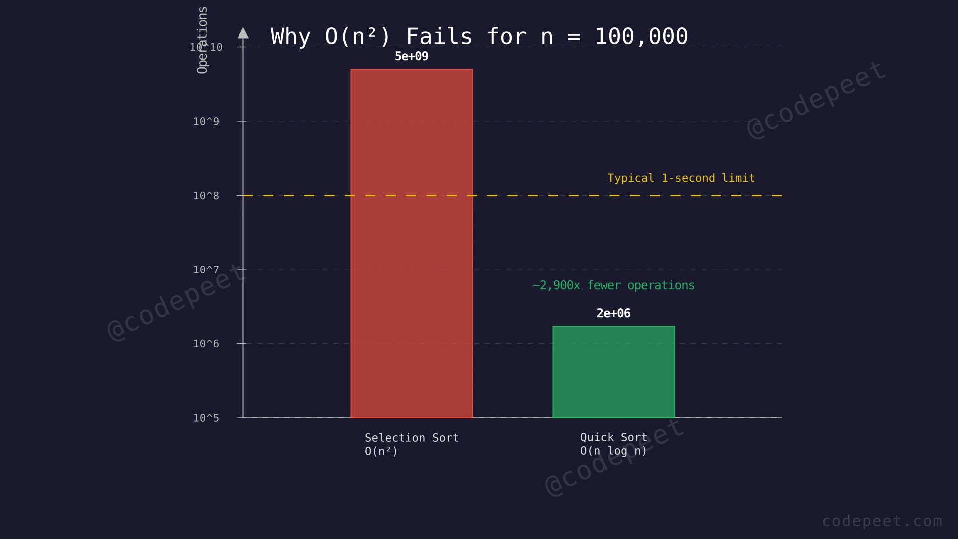
Selection sort (and other O(n²) algorithms like bubble sort and insertion sort) are too slow for the given constraints. With n up to 10^5, an O(n²) algorithm performs up to 5 × 10^9 operations — far exceeding the typical time limit.
The fundamental problem: these algorithms make one placement per pass and each pass requires scanning all remaining elements. They never divide the problem into independent subproblems that can be solved separately.
The key insight for a faster approach: divide and conquer. Instead of placing one element at a time, what if we could split the array into two halves around a pivot element, so that everything on the left is smaller and everything on the right is larger? Then each half can be sorted independently. If the split is roughly balanced, we reduce the problem size by half at each level, giving O(n log n) performance.
This is exactly what Quick Sort does — and the partition step that achieves this split runs in just O(n) time.
Optimal Approach - Quick Sort (Lomuto Partition)
Intuition
Quick Sort is a divide-and-conquer algorithm built around a clever operation called partitioning.
Imagine you are a teacher sorting students by height. Instead of comparing every pair (O(n²)), you try a smarter strategy: you pick one student as a reference (the pivot). You ask all shorter students to stand on the left, and all taller students on the right. Now the reference student is in their exact correct position — everyone shorter is to their left, everyone taller is to their right.
You then ask two assistant teachers to repeat this same process independently on the left group and the right group. Each assistant picks a reference from their group, splits it, and delegates further. This continues until groups have just one student (trivially sorted).
The Lomuto Partition Scheme is a specific way to perform the partition step:
- Choose the last element as the pivot
- Maintain a boundary pointer
ithat tracks where the next "small" element should go - Scan from left to right with pointer
j:- If
arr[j]is less than the pivot, swap it witharr[i]and advancei - Otherwise, skip it
- If
- After the scan, swap the pivot (at the end) with
arr[i+1]to place it in its correct position - Return
i+1as the pivot's final index
After partitioning, elements at indices 0..pivot-1 are all ≤ pivot, and elements at indices pivot+1..n-1 are all > pivot. We then recursively sort both halves.
Step-by-Step Explanation
Let's trace the first partition call on arr = [4, 1, 3, 9, 7], with low=0 and high=4:
Pivot = arr[4] = 7. Initialize i = low - 1 = -1.
Step 1: j=0, arr[0]=4. Is 4 < 7? YES. Increment i to 0. Swap arr[0] with arr[0] (no change). Array: [4, 1, 3, 9, 7]. i=0.
Step 2: j=1, arr[1]=1. Is 1 < 7? YES. Increment i to 1. Swap arr[1] with arr[1] (no change). Array: [4, 1, 3, 9, 7]. i=1.
Step 3: j=2, arr[2]=3. Is 3 < 7? YES. Increment i to 2. Swap arr[2] with arr[2] (no change). Array: [4, 1, 3, 9, 7]. i=2.
Step 4: j=3, arr[3]=9. Is 9 < 7? NO. Do nothing. i stays at 2.
Step 5: Loop ends. Swap pivot arr[4]=7 with arr[i+1]=arr[3]=9. Array becomes [4, 1, 3, 7, 9]. Pivot 7 is now at index 3 — its correct sorted position!
After partition: [4, 1, 3 | 7 | 9]. Left subarray [4, 1, 3] needs sorting. Right subarray [9] has one element (already sorted).
Recurse on left subarray [4, 1, 3] (low=0, high=2):
Pivot = arr[2] = 3. i = -1.
Step 6: j=0, arr[0]=4. Is 4 < 3? NO. Skip. i stays -1.
Step 7: j=1, arr[1]=1. Is 1 < 3? YES. Increment i to 0. Swap arr[0]=4 with arr[0+0]... wait — swap arr[i]=arr[0] with arr[j]=arr[1]: array becomes [1, 4, 3, 7, 9]. i=0.
Step 8: Loop ends. Swap pivot arr[2]=3 with arr[i+1]=arr[1]=4. Array becomes [1, 3, 4, 7, 9]. Pivot 3 at index 1.
After this partition: [1 | 3 | 4, 7, 9]. Left [1] and right [4] are single elements.
Result: [1, 3, 4, 7, 9]
Quick Sort — Lomuto Partition on [4, 1, 3, 9, 7] — Watch the Lomuto partition scheme place the pivot (last element) in its correct position by scanning left-to-right and swapping smaller elements to the front.
Algorithm
partition(arr, low, high):
- Choose pivot = arr[high] (last element)
- Set i = low - 1 (boundary of elements less than pivot)
- For j from low to high - 1:
- If arr[j] < pivot:
- Increment i
- Swap arr[i] and arr[j]
- If arr[j] < pivot:
- Swap arr[i + 1] and arr[high] (place pivot in correct position)
- Return i + 1 (pivot's final index)
quickSort(arr, low, high):
- If low < high:
- pi = partition(arr, low, high)
- quickSort(arr, low, pi - 1) — sort left subarray
- quickSort(arr, pi + 1, high) — sort right subarray
Code
#include <vector>
using namespace std;

class Solution {
public:
    int partition(vector<int>& arr, int low, int high) {
        int pivot = arr[high];
        int i = low - 1;

        for (int j = low; j < high; j++) {
            if (arr[j] < pivot) {
                i++;
                swap(arr[i], arr[j]);
            }
        }

        swap(arr[i + 1], arr[high]);
        return i + 1;
    }

    void quickSort(vector<int>& arr, int low, int high) {
        if (low < high) {
            int pi = partition(arr, low, high);
            quickSort(arr, low, pi - 1);
            quickSort(arr, pi + 1, high);
        }
    }

    void quickSort(vector<int>& arr) {
        quickSort(arr, 0, arr.size() - 1);
    }
};
class Solution:
def partition(self, arr: list[int], low: int, high: int) -> int:
pivot = arr[high]
i = low - 1
for j in range(low, high):
if arr[j] < pivot:
i += 1
arr[i], arr[j] = arr[j], arr[i]
arr[i + 1], arr[high] = arr[high], arr[i + 1]
return i + 1
def quickSort(self, arr: list[int], low: int, high: int) -> None:
if low < high:
pi = self.partition(arr, low, high)
self.quickSort(arr, low, pi - 1)
self.quickSort(arr, pi + 1, high)class Solution {
int partition(int[] arr, int low, int high) {
int pivot = arr[high];
int i = low - 1;
for (int j = low; j < high; j++) {
if (arr[j] < pivot) {
i++;
int temp = arr[i];
arr[i] = arr[j];
arr[j] = temp;
}
}
int temp = arr[i + 1];
arr[i + 1] = arr[high];
arr[high] = temp;
return i + 1;
}
void quickSort(int[] arr, int low, int high) {
if (low < high) {
int pi = partition(arr, low, high);
quickSort(arr, low, pi - 1);
quickSort(arr, pi + 1, high);
}
}
}Complexity Analysis
Time Complexity:
-
Best Case: O(n log n) — Occurs when the pivot always divides the array into two roughly equal halves. Each level of recursion processes all n elements (for partitioning), and there are log n levels. Total: O(n × log n).
-
Average Case: O(n log n) — On average, the pivot creates reasonably balanced partitions. Mathematical analysis shows the expected number of comparisons is approximately 1.39 × n × log₂(n).
-
Worst Case: O(n²) — Occurs when the pivot is always the smallest or largest element (e.g., array is already sorted and we pick the last element as pivot). Each partition only reduces the problem size by 1, leading to n levels of recursion with O(n) work each. Total: O(n²).
Space Complexity:
-
Best/Average Case: O(log n) — The recursion stack depth is proportional to the depth of the recursion tree, which is O(log n) for balanced partitions.
-
Worst Case: O(n) — When partitions are maximally unbalanced, the recursion depth reaches n, requiring O(n) stack space.
Despite the O(n²) worst case, quick sort is often the fastest sorting algorithm in practice due to its excellent cache performance, low constant factors, and the rarity of the worst case with good pivot selection strategies.