Complexity Analysis Primer
Description
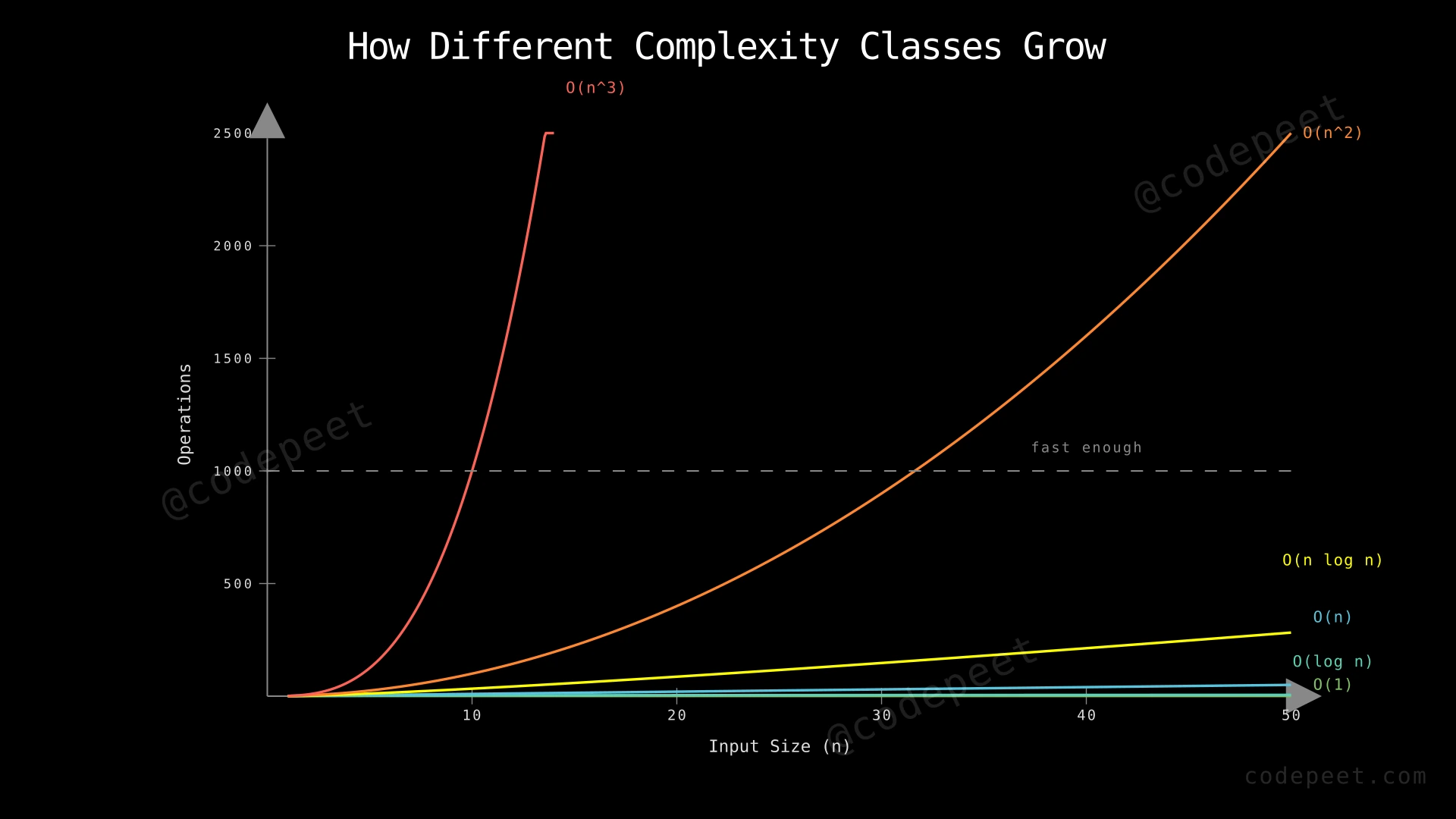
Time complexity is a way to describe how the running time of an algorithm grows as the size of its input increases. Rather than measuring the actual seconds a program takes (which depends on hardware, operating system load, and other factors), we measure the number of fundamental operations an algorithm performs as a function of the input size n.
Your task is to understand, analyze, and determine the time complexity of simple code snippets involving loops and basic operations. Given a code fragment, identify its Big-O time complexity and explain your reasoning.
This is a foundational concept — every algorithm you will ever study or write has a time complexity, and understanding it is the first step to writing efficient code.
Examples
Example 1
Input: A code snippet that prints "Hello" once.
print("Hello")
Output: O(1)
Explanation: The code executes a single statement regardless of any input size. Whether you call this function once or define n to be a million, this line always runs exactly once. This is called constant time complexity.
Example 2
Input: A code snippet that iterates through an array of size n.
for i in range(n):
    print(arr[i])
Output: O(n)
Explanation: The loop runs exactly n times — once for each element in the array. If the array has 10 elements, it runs 10 times. If it has 1,000,000 elements, it runs 1,000,000 times. The number of operations grows linearly with n, giving us linear time complexity O(n).
Example 3
Input: A code snippet with nested loops.
for i in range(n):
    for j in range(n):
        print(i, j)
Output: O(n²)
Explanation: The outer loop runs n times. For each iteration of the outer loop, the inner loop also runs n times. So the total number of print operations is n × n = n². If n = 10, there are 100 operations. If n = 1000, there are 1,000,000 operations. The growth is quadratic.
Example 4
Input: A code snippet where the loop variable is halved each time.
i = n
while i > 0:
    print(i)
    i = i // 2
Output: O(log n)
Explanation: The variable i starts at n and is halved each iteration. It takes roughly log₂(n) halvings before i reaches 0. For n = 16, the iterations are: 16 → 8 → 4 → 2 → 1 → 0, which is 5 iterations ≈ log₂(16) + 1. This is logarithmic time complexity.
Constraints
- 1 ≤ n ≤ 10^9 (input size can be very large)
- Code snippets involve basic operations: arithmetic, comparisons, assignments
- Loops may be simple (single), nested, or involve multiplicative/divisive step changes
- We analyze worst-case time complexity using Big-O notation
- Constants and lower-order terms are dropped (e.g., 3n + 5 becomes O(n))
Editorial
Brute Force
Intuition
The most straightforward way to determine time complexity is the counting approach: manually count how many times each statement executes, sum them all up, and simplify.
Imagine you are a teacher grading papers. If you have one paper, it takes a fixed amount of time. If you have n papers, you spend time proportional to n. If for every paper you also compare it with every other paper for plagiarism, that is n × n comparisons. The counting approach is like literally writing down every single operation and adding them up.
This works perfectly for simple code, but becomes tedious and error-prone for complex programs. It is the brute force of complexity analysis — correct but inefficient for the analyst.
Step-by-Step Explanation
Let's analyze the time complexity of finding the sum of an array by counting every single operation:
sum = 0               // Line A
for i = 0 to n-1:     // Line B
    sum = sum + arr[i] // Line C
return sum             // Line D
Step 1: Line A executes once → 1 operation (assignment).
Step 2: Line B: The loop initialization i = 0 executes once → 1 operation.
Step 3: Line B: The loop condition i < n is checked n+1 times (n times it is true, once it is false to exit) → n+1 operations.
Step 4: Line B: The increment i++ executes n times → n operations.
Step 5: Line C: The addition sum + arr[i] and assignment execute n times → 2n operations (one add + one assign per iteration).
Step 6: Line D executes once → 1 operation.
Step 7: Total count = 1 + 1 + (n+1) + n + 2n + 1 = 4n + 4.
Step 8: Drop constants and lower-order terms: 4n + 4 → O(n).
The counting approach gives us the exact expression 4n + 4, but we only care about the growth rate, so we simplify to O(n).
Counting Operations — Array Sum Analysis — Watch how we count every individual operation as the loop processes each element of the array, building up to the total operation count.
Algorithm
- For each line of code, count how many times it executes as a function of
n - Multiply the count by the cost of each operation (assume constant cost per operation)
- Sum all the individual counts to get a total expression like
4n + 4 - Identify the highest-order term (the term that grows fastest as n increases)
- Drop all constants and lower-order terms
- Express the result in Big-O notation: O(highest-order term)
Code
#include <iostream>
#include <vector>
using namespace std;

// Demonstrates O(n) — count every operation
int arraySum(vector<int>& arr) {
    int n = arr.size();       // 1 operation
    int sum = 0;              // 1 operation
    for (int i = 0; i < n; i++) {  // init: 1, compare: n+1, increment: n
        sum = sum + arr[i];   // 2n operations (add + assign)
    }
    return sum;               // 1 operation
    // Total: 4n + 4 => O(n)
}
# Demonstrates O(n) — count every operation
def array_sum(arr):
n = len(arr) # 1 operation
total = 0 # 1 operation
for i in range(n): # loop runs n times
total += arr[i] # 1 add + 1 assign = 2 ops per iteration
return total # 1 operation
# Total: ~2n + 3 => O(n)class Solution {
// Demonstrates O(n) — count every operation
public int arraySum(int[] arr) {
int n = arr.length; // 1 operation
int sum = 0; // 1 operation
for (int i = 0; i < n; i++) { // init: 1, compare: n+1, incr: n
sum = sum + arr[i]; // 2n operations
}
return sum; // 1 operation
// Total: 4n + 4 => O(n)
}
}Complexity Analysis
Time Complexity of the Counting Approach: O(n) for simple single-loop code.
We manually counted every operation and arrived at 4n + 4. The dominant term is 4n, which simplifies to O(n). The constant factors (4 and 4) do not matter in Big-O because they don't change the fundamental growth rate — whether the exact count is 4n or 100n, it still grows linearly with n.
Space Complexity: O(1)
The counting approach itself uses no extra space beyond a few variables. The sum variable and loop counter are constant regardless of input size.
Limitation of this approach: While accurate, manually counting every operation becomes extremely tedious for code with multiple nested loops, recursive calls, or conditional branches. For a nested loop with complex logic, you might need to count dozens of operation types — this is error-prone and slow for the analyst.
Why This Approach Is Not Efficient
The brute-force counting method works, but it has significant drawbacks:
-
It's tedious: For a doubly nested loop, you need to track initialization, condition checks, increments, and body operations for both loops — easily 8+ terms to sum.
-
Constants don't matter: Whether the exact count is 4n + 4 or 7n + 12, both simplify to O(n). Spending time computing the exact constant is wasted effort.
-
It doesn't scale to complex code: Recursive algorithms, algorithms with conditional branches, or code that calls other functions make manual counting impractical.
The key insight is: we only care about the dominant term. Instead of counting every single operation, we can directly identify which loop or structure determines the growth rate. If there is a single loop running n times with constant work inside, it is O(n) — period. No need to count whether it is 3n or 5n operations.
This leads us to a better approach: analyzing the loop structure directly.
Better Approach - Loop Structure Analysis
Intuition
Instead of counting every operation, focus on the structure of loops:
- No loop? → O(1) — constant time, happens once regardless of input.
- One loop from 0 to n? → O(n) — the loop body executes proportionally to n.
- Two nested loops, each going to n? → O(n²) — the inner body runs n × n times.
- Loop variable doubles or halves? → O(log n) — the loop terminates after logarithmically many steps.
Think of it like estimating travel time. You don't need to count every step you take from your house to the store. You just need to know the distance (1 km) and your walking speed (5 km/h) to estimate it will take about 12 minutes. Similarly, the loop structure tells you the "distance" (how many iterations), and the body tells you the "speed" (constant work per iteration).
Step-by-Step Explanation
Let's analyze four different code patterns using loop structure analysis:
Code A — Constant Time O(1):
a = 5
b = a + 10
print(b)
Step 1: No loops present. All statements execute exactly once. Answer: O(1).
Code B — Linear Time O(n):
for i in range(n):
    print(i)
Step 2: One loop running from 0 to n-1. Body does constant work (one print). Loop runs n times × O(1) work = O(n).
Code C — Quadratic Time O(n²):
for i in range(n):
    for j in range(n):
        print(i, j)
Step 3: Outer loop runs n times. For each outer iteration, inner loop runs n times. Body does O(1). Total: n × n × O(1) = O(n²).
Code D — Logarithmic Time O(log n):
i = n
while i >= 1:
    print(i)
    i = i // 2
Step 4: Loop variable starts at n and halves each iteration. Number of halvings to reach 1 from n is log₂(n). Body does O(1). Total: O(log n).
Step 5: Compare growth rates for n = 1000: O(1) = 1 op, O(log n) ≈ 10 ops, O(n) = 1000 ops, O(n²) = 1,000,000 ops.
Step 6: The loop structure directly tells you the complexity class without counting individual operations.
Loop Structure Analysis — Comparing Four Complexity Classes — Watch how four different loop patterns produce dramatically different operation counts for the same input size n=8, revealing the power of structural analysis.
Algorithm
- Identify the loop structure in the code:
- No loop → O(1)
- Single loop incrementing by a constant (i++, i+=c) → O(n)
- Single loop multiplying/dividing by a constant (i*=2, i/=2) → O(log n)
- Two nested loops, each running n times → O(n²)
- Three nested loops, each running n times → O(n³)
- If there are consecutive (non-nested) loops, take the maximum: O(n) + O(n²) = O(n²)
- If the inner loop depends on the outer variable, analyze the total number of inner iterations across all outer iterations
- Drop constants and lower-order terms from the final expression
Code
#include <iostream>
#include <vector>
using namespace std;

// O(1) — Constant: no loop
int constantExample(int a, int b) {
    return a + b;
}

// O(log n) — Logarithmic: halving loop
int logExample(int n) {
    int count = 0;
    for (int i = n; i >= 1; i /= 2) {
        count++;
    }
    return count; // returns ~log2(n)
}

// O(n) — Linear: single loop
int linearExample(vector<int>& arr) {
    int sum = 0;
    for (int i = 0; i < arr.size(); i++) {
        sum += arr[i];
    }
    return sum;
}

// O(n^2) — Quadratic: nested loops
int quadraticExample(vector<int>& arr) {
    int n = arr.size();
    int pairCount = 0;
    for (int i = 0; i < n; i++) {
        for (int j = i + 1; j < n; j++) {
            pairCount++;
        }
    }
    return pairCount; // returns n*(n-1)/2
}
# O(1) — Constant: no loop
def constant_example(a, b):
return a + b
# O(log n) — Logarithmic: halving loop
def log_example(n):
count = 0
i = n
while i >= 1:
count += 1
i //= 2
return count # returns ~log2(n)
# O(n) — Linear: single loop
def linear_example(arr):
total = 0
for num in arr:
total += num
return total
# O(n^2) — Quadratic: nested loops
def quadratic_example(arr):
n = len(arr)
pair_count = 0
for i in range(n):
for j in range(i + 1, n):
pair_count += 1
return pair_count # returns n*(n-1)//2class Solution {
// O(1) — Constant: no loop
public int constantExample(int a, int b) {
return a + b;
}
// O(log n) — Logarithmic: halving loop
public int logExample(int n) {
int count = 0;
for (int i = n; i >= 1; i /= 2) {
count++;
}
return count; // returns ~log2(n)
}
// O(n) — Linear: single loop
public int linearExample(int[] arr) {
int sum = 0;
for (int i = 0; i < arr.length; i++) {
sum += arr[i];
}
return sum;
}
// O(n^2) — Quadratic: nested loops
public int quadraticExample(int[] arr) {
int n = arr.length;
int pairCount = 0;
for (int i = 0; i < n; i++) {
for (int j = i + 1; j < n; j++) {
pairCount++;
}
}
return pairCount; // returns n*(n-1)/2
}
}Complexity Analysis
Analysis Speed: The loop structure approach is much faster for the analyst — you can determine complexity by visual inspection in seconds rather than manually counting dozens of operations.
The four complexity classes identified:
- O(1): No loop or loop runs a fixed number of times. Execution time is independent of input size.
- O(log n): Loop variable multiplied or divided by a constant each iteration. Takes log₂(n) steps because you need log₂(n) halvings to go from n down to 1.
- O(n): Loop variable incremented/decremented by a constant. Visits each of the n elements once.
- O(n²): Two nested loops, each proportional to n. The inner loop runs n times for each of the n outer iterations, yielding n × n = n² total body executions.
Space Complexity: O(1) for all examples. Each uses only a fixed number of variables regardless of input size.
Limitation: This approach handles standard loop patterns well, but can struggle with tricky cases like loops where the inner range depends on the outer variable in non-obvious ways, or recursive algorithms where the number of calls forms a tree. For those, we need a more systematic approach.
Why This Approach Is Not Efficient
The loop structure approach handles the four standard patterns (constant, logarithmic, linear, quadratic) very well. However, it struggles with more subtle scenarios:
-
Dependent inner loops: When the inner loop range depends on the outer variable (e.g.,
for j in range(i)), the total iterations are not simply n × n. You need to sum a series: 0 + 1 + 2 + ... + (n-1) = n(n-1)/2 = O(n²). Knowing this requires recognizing arithmetic series. -
Consecutive loops: If code has a loop running n times followed by a nested loop running n², the total is O(n) + O(n²) = O(n²). You need to know that the dominant term wins.
-
Logarithmic variations: A loop where i goes 1, 2, 4, 8, ... n is O(log n), but what about
for i = 2 to n, i = i*i? That is O(log log n). Pattern recognition alone may miss these. -
Recursive algorithms: Recursion trees and the Master Theorem handle cases where a function calls itself multiple times with smaller inputs.
To handle all these cases confidently, we need a systematic framework — a set of rules and formulas that cover every common pattern.
Optimal Approach - Systematic Complexity Rules
Intuition
The optimal approach is to internalize a small set of rules that cover virtually all common code patterns. Instead of counting operations or guessing from loop shapes, you apply these rules mechanically:
Rule 1 — Sequential Composition: If two blocks of code run one after another, the total complexity is the maximum of the two. O(n) followed by O(n²) = O(n²). Think of it as: the slower step dominates.
Rule 2 — Nested Multiplication: If an inner loop runs inside an outer loop, multiply their complexities. An O(n) loop containing an O(n) loop = O(n × n) = O(n²).
Rule 3 — Logarithmic Detection: If a loop variable is multiplied or divided by a constant (i *= 2, i /= 3), the loop runs O(log n) times.
Rule 4 — Dependent Inner Loops (Series Summation): If the inner loop runs i times and i goes from 1 to n, sum the series: 1 + 2 + ... + n = n(n+1)/2 = O(n²).
Rule 5 — Drop Constants and Lower Terms: 3n² + 7n + 15 → O(n²). Only the fastest-growing term matters.
With these five rules, you can analyze nearly any iterative algorithm in seconds.
Step-by-Step Explanation
Let's apply the systematic rules to analyze a tricky code snippet:
for i in range(n):           // Loop 1: outer
    for j in range(i):       // Loop 2: inner (depends on i)
        print(i, j)

for k in range(n):           // Loop 3: separate
    print(k)
Step 1: Identify the structure — two blocks: (a) nested loops, (b) single loop. By Rule 1, total = max(block_a, block_b).
Step 2: Analyze block (b) first (easy): Loop 3 runs n times with O(1) body → O(n).
Step 3: Analyze block (a) — the nested loops. The inner loop runs i times, where i goes from 0 to n-1. By Rule 4 (dependent inner loop), we sum: 0 + 1 + 2 + ... + (n-1).
Step 4: Compute the sum using the arithmetic series formula: sum = n(n-1)/2.
Step 5: Expand: n(n-1)/2 = (n² - n) / 2. Apply Rule 5 (drop constants and lower terms): O(n²).
Step 6: Apply Rule 1 (sequential composition): max(O(n²), O(n)) = O(n²).
Step 7: Final answer: O(n²). The nested dependent loop dominates the single loop.
Step 8: Verify with n = 4: inner iterations = 0+1+2+3 = 6, plus loop 3 = 4 iterations. Total body executions = 10. Formula: 4(3)/2 + 4 = 6 + 4 = 10. As n grows, the n²/2 term dominates.
Systematic Rules — Analyzing Dependent Nested Loops — Watch how we apply the series summation rule to count total iterations when the inner loop depends on the outer variable, then combine with the sequential composition rule.
Algorithm
The Systematic Complexity Analysis Framework:
- Identify all loops and their nesting structure
- For each loop, determine its type:
- Constant iterations (fixed number) → contributes O(1)
- Linear iterations (increment by constant, i++, i+=c) → contributes O(n)
- Logarithmic iterations (multiply/divide by constant, i*=2, i/=2) → contributes O(log n)
- For nested loops, apply Rule 2: Multiply complexities of nested levels
- For dependent inner loops, apply Rule 4: Sum the series of inner iterations
- i from 1 to n, inner runs i times → sum = n(n+1)/2 → O(n²)
- i from 1 to n, inner runs n/i times → sum ≈ n·ln(n) → O(n log n)
- For consecutive (sequential) blocks, apply Rule 1: Take the maximum
- Apply Rule 5: Drop all constants and lower-order terms from the final expression
- Express in Big-O notation: O(dominant term)
Code
#include <iostream>
using namespace std;

// Example: Dependent inner loop → O(n^2)
// Demonstrates Rule 4 (series summation)
void dependentLoopExample(int n) {
    int count = 0;
    for (int i = 0; i < n; i++) {       // Outer: n iterations
        for (int j = 0; j < i; j++) {   // Inner: i iterations (depends on outer)
            count++;                     // Total: 0+1+2+...+(n-1) = n(n-1)/2
        }
    }
    cout << "Total operations: " << count << endl;
    // count = n*(n-1)/2 => O(n^2)
}

// Example: Sequential composition → O(n^2)
// Demonstrates Rule 1 (max of sequential blocks)
void sequentialExample(int n) {
    // Block A: O(n)
    for (int i = 0; i < n; i++) {
        cout << i << " ";
    }

    // Block B: O(n^2)
    for (int i = 0; i < n; i++) {
        for (int j = 0; j < n; j++) {
            cout << i * j << " ";
        }
    }
    // Total: max(O(n), O(n^2)) = O(n^2)
}

// Example: O(n log n) — log inner inside linear outer
void nLogNExample(int n) {
    int count = 0;
    for (int i = 0; i < n; i++) {       // Outer: O(n)
        for (int j = 1; j < n; j *= 2) { // Inner: O(log n)
            count++;
        }
    }
    cout << "Total: " << count << endl;
    // Total: n * log(n) => O(n log n)
}
# Example: Dependent inner loop → O(n^2)
# Demonstrates Rule 4 (series summation)
def dependent_loop_example(n):
count = 0
for i in range(n): # Outer: n iterations
for j in range(i): # Inner: i iterations (depends on outer)
count += 1 # Total: 0+1+2+...+(n-1) = n(n-1)/2
print(f"Total operations: {count}")
# count = n*(n-1)//2 => O(n^2)
# Example: Sequential composition → O(n^2)
# Demonstrates Rule 1 (max of sequential blocks)
def sequential_example(n):
# Block A: O(n)
for i in range(n):
print(i, end=" ")
# Block B: O(n^2)
for i in range(n):
for j in range(n):
print(i * j, end=" ")
# Total: max(O(n), O(n^2)) = O(n^2)
# Example: O(n log n) — log inner inside linear outer
def n_log_n_example(n):
count = 0
for i in range(n): # Outer: O(n)
j = 1
while j < n: # Inner: O(log n)
count += 1
j *= 2
print(f"Total: {count}")
# Total: n * log(n) => O(n log n)class Solution {
// Example: Dependent inner loop → O(n^2)
// Demonstrates Rule 4 (series summation)
public void dependentLoopExample(int n) {
int count = 0;
for (int i = 0; i < n; i++) { // Outer: n iterations
for (int j = 0; j < i; j++) { // Inner: i iterations
count++; // Total: 0+1+...+(n-1) = n(n-1)/2
}
}
System.out.println("Total operations: " + count);
// count = n*(n-1)/2 => O(n^2)
}
// Example: Sequential composition → O(n^2)
// Demonstrates Rule 1 (max of sequential blocks)
public void sequentialExample(int n) {
// Block A: O(n)
for (int i = 0; i < n; i++) {
System.out.print(i + " ");
}
// Block B: O(n^2)
for (int i = 0; i < n; i++) {
for (int j = 0; j < n; j++) {
System.out.print(i * j + " ");
}
}
// Total: max(O(n), O(n^2)) = O(n^2)
}
// Example: O(n log n) — log inner inside linear outer
public void nLogNExample(int n) {
int count = 0;
for (int i = 0; i < n; i++) { // Outer: O(n)
for (int j = 1; j < n; j *= 2) { // Inner: O(log n)
count++;
}
}
System.out.println("Total: " + count);
// Total: n * log(n) => O(n log n)
}
}Complexity Analysis
The Systematic Rules Framework covers all common iterative patterns:
Summary of Rules and Their Applications:
| Rule | Pattern | Result | Example |
|---|---|---|---|
| Sequential (Rule 1) | A then B | max(A, B) | O(n) + O(n²) = O(n²) |
| Nesting (Rule 2) | A inside B | A × B | O(n) × O(n) = O(n²) |
| Logarithmic (Rule 3) | i *= c or i /= c | O(log n) | while(i < n) i *= 2 |
| Series (Rule 4) | inner = f(outer) | sum the series | Σi from 0 to n-1 = O(n²) |
| Simplify (Rule 5) | Drop constants | Keep dominant term | 5n² + 3n → O(n²) |
Common Complexity Hierarchy (from fastest to slowest):
O(1) < O(log n) < O(√n) < O(n) < O(n log n) < O(n²) < O(n³) < O(2ⁿ) < O(n!)
Practical Guideline for Competitive Programming:
- n ≤ 10: O(n!) is acceptable
- n ≤ 20: O(2ⁿ) is acceptable
- n ≤ 500: O(n³) is acceptable
- n ≤ 10,000: O(n²) is acceptable
- n ≤ 1,000,000: O(n log n) is acceptable
- n ≤ 100,000,000: O(n) is needed
Space Complexity: The analysis framework itself uses O(1) space — it is a mental/analytical process, not an algorithm that consumes memory.
With these five rules, you can confidently determine the time complexity of any iterative code you encounter in interviews or coursework.