Introduction to Dynamic Programming
Description
Dynamic Programming (DP) is a method for solving complex problems by breaking them into smaller, overlapping subproblems and storing their results to avoid redundant computation. It transforms recursive solutions that take exponential time into efficient ones that run in polynomial time.
To introduce DP, we use the classic Fibonacci number problem:
Given an integer n, compute the nth Fibonacci number. The Fibonacci sequence is defined as:
- F(0) = 0
- F(1) = 1
- F(n) = F(n - 1) + F(n - 2) for n ≥ 2
The sequence begins: 0, 1, 1, 2, 3, 5, 8, 13, 21, 34, ...
This seemingly simple problem perfectly illustrates why DP exists: the naive recursive approach is catastrophically slow, but with DP techniques (memoization or tabulation), it becomes trivially fast. Two key properties make a problem suitable for DP:
- Overlapping Subproblems: The same subproblem is solved multiple times during recursion. For Fibonacci, computing F(5) requires F(3) twice and F(2) three times.
- Optimal Substructure: The solution to the overall problem can be constructed from solutions to its subproblems. F(n) is directly built from F(n-1) and F(n-2).
Examples
Example 1
Input: n = 5
Output: 5
Explanation: The Fibonacci sequence up to index 5 is: F(0)=0, F(1)=1, F(2)=1, F(3)=2, F(4)=3, F(5)=5. We compute F(5) = F(4) + F(3) = 3 + 2 = 5.
Example 2
Input: n = 0
Output: 0
Explanation: F(0) = 0 is a base case of the Fibonacci definition. No computation is needed beyond returning the base value.
Example 3
Input: n = 10
Output: 55
Explanation: The Fibonacci sequence: 0, 1, 1, 2, 3, 5, 8, 13, 21, 34, 55. F(10) = F(9) + F(8) = 34 + 21 = 55. Without DP, naive recursion would make 177 function calls for this input. With DP, we need only 11 computations.
Constraints
- 0 ≤ n ≤ 30
- The answer fits in a 32-bit signed integer
Editorial
Brute Force
Intuition
The most direct way to compute Fibonacci is to translate the mathematical definition straight into code: F(n) = F(n-1) + F(n-2), with base cases F(0) = 0 and F(1) = 1.
This gives us a recursive function. When we call fib(5), it calls fib(4) and fib(3). Then fib(4) calls fib(3) and fib(2), and so on, until we reach the base cases. The function then bubbles results upward.
The problem is hidden in the recursion tree: the same subproblem is computed over and over again. For instance, fib(3) is computed once by fib(5) and again by fib(4). fib(2) is computed even more times. This duplication grows exponentially — which is exactly why this approach fails for anything beyond small inputs.
Step-by-Step Explanation
Let's trace the recursive computation of fib(5):
Step 1: Call fib(5). It needs fib(4) and fib(3). Start with the left branch: fib(4).
Step 2: Call fib(4). It needs fib(3) and fib(2). Recurse into fib(3).
Step 3: Call fib(3). It needs fib(2) and fib(1). Recurse into fib(2).
Step 4: Call fib(2). It needs fib(1)=1 and fib(0)=0. Both are base cases. fib(2) = 1 + 0 = 1.
Step 5: Back to fib(3). Its right child is fib(1) = 1 (base case). fib(3) = fib(2) + fib(1) = 1 + 1 = 2.
Step 6: Back to fib(4). Its right child is fib(2) — but we already computed this in Step 4! The naive approach does NOT remember, so it recomputes from scratch: fib(2) = 1.
Step 7: fib(4) = fib(3) + fib(2) = 2 + 1 = 3.
Step 8: Back to fib(5). Its right child is fib(3) — already computed in Steps 3-5! Again, the naive approach recomputes the entire subtree: fib(3) = 2.
Step 9: fib(5) = fib(4) + fib(3) = 3 + 2 = 5. Total function calls: 15. For fib(5), the tree has 15 nodes instead of the 6 unique subproblems.
Naive Recursion — Exponential Explosion of Overlapping Calls — Watch the recursion tree grow as fib(5) spawns redundant subtrees. The same subproblems (highlighted) are recomputed from scratch each time.
Algorithm
- If n is 0, return 0 (base case)
- If n is 1, return 1 (base case)
- Recursively compute fib(n - 1)
- Recursively compute fib(n - 2)
- Return fib(n - 1) + fib(n - 2)
Code
#include <iostream>
using namespace std;

class Solution {
public:
    int fib(int n) {
        if (n == 0) return 0;
        if (n == 1) return 1;
        return fib(n - 1) + fib(n - 2);
    }
};
class Solution:
def fib(self, n: int) -> int:
if n == 0:
return 0
if n == 1:
return 1
return self.fib(n - 1) + self.fib(n - 2)class Solution {
public int fib(int n) {
if (n == 0) return 0;
if (n == 1) return 1;
return fib(n - 1) + fib(n - 2);
}
}Complexity Analysis
Time Complexity: O(2^n)
Each call branches into two sub-calls, creating a binary tree of depth n. The total number of nodes in this tree is approximately 2^n. More precisely, the number of calls is equal to 2×F(n+1) - 1, which grows exponentially at a rate of roughly φ^n (where φ ≈ 1.618 is the golden ratio).
Space Complexity: O(n)
The maximum depth of the recursion stack is n, since the deepest call chain is fib(n) → fib(n-1) → ... → fib(1). Each frame on the stack uses O(1) space, giving O(n) total stack space.
Why This Approach Is Not Efficient
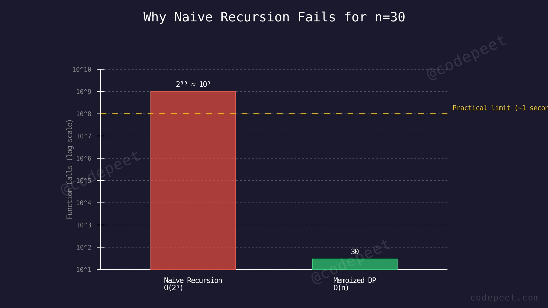
The naive recursion runs in O(2^n) time. For n = 30, this means over 1 billion function calls. For n = 50, we would need roughly 10^15 calls — that would take thousands of years on any modern computer.
The root cause is overlapping subproblems: the recursion tree recomputes the same Fibonacci values over and over. fib(2) alone is computed F(n-1) times. There are only n+1 unique subproblems (fib(0) through fib(n)), yet the naive approach solves an exponential number of subproblem instances.
Key insight — Memoization: If we store ("memoize") the result of each subproblem the first time we compute it, we can simply look it up on subsequent calls. This eliminates ALL redundant work, since each of the n+1 subproblems is computed exactly once. The time drops from O(2^n) to O(n) — an astronomical improvement.
Better Approach - Memoization (Top-Down DP)
Intuition
Memoization is the simplest fix for the overlapping subproblems issue. The idea is: keep the same recursive structure, but add a lookup table (the "memo"). Before computing any subproblem, first check if the answer is already in the memo. If yes, return it immediately. If no, compute it normally, store the result in the memo, and then return it.
Think of it like a student doing homework. Without memoization, every time the teacher asks 'What is 7 × 8?', the student multiplies from scratch. With memoization, the student writes the answer on a sticky note the first time. Every subsequent question of '7 × 8?' gets answered instantly by reading the note.
This approach is called top-down because we start from the original problem (fib(n)) and work our way down to base cases, taking shortcuts whenever we encounter a previously solved subproblem.
Step-by-Step Explanation
Let's trace fib(5) with memoization (memo initially empty):
Step 1: Call fib(5). Memo empty. Recurse into fib(4).
Step 2: Call fib(4). Memo empty. Recurse into fib(3).
Step 3: Call fib(3). Memo empty. Recurse into fib(2).
Step 4: Call fib(2). Memo empty. Reach base cases: fib(1)=1, fib(0)=0. fib(2) = 1. Store memo[2] = 1.
Step 5: Back to fib(3). Call fib(1)=1 (base case). fib(3) = fib(2)+fib(1) = 1+1 = 2. Store memo[3] = 2.
Step 6: Back to fib(4). Call fib(2) — CHECK MEMO — FOUND! memo[2]=1. Return immediately. No subtree needed! This saves 2 function calls.
Step 7: fib(4) = fib(3)+fib(2) = 2+1 = 3. Store memo[4] = 3.
Step 8: Back to fib(5). Call fib(3) — CHECK MEMO — FOUND! memo[3]=2. Return immediately. This saves 4 function calls (the entire fib(3) subtree).
Step 9: fib(5) = fib(4)+fib(3) = 3+2 = 5. Store memo[5] = 5. Total: only 9 calls instead of 15.
Memoization — Pruning Redundant Subtrees with a Lookup Table — Watch how the memo table prevents redundant computations. When a subproblem is encountered again, it returns instantly (shown as pruned nodes) instead of spawning an entire subtree.
Algorithm
- Create a memo array of size n+1, initialized to -1 (meaning "not yet computed")
- Define a recursive helper function fibMemo(k, memo):
a. If k ≤ 1, return k (base case)
b. If memo[k] ≠ -1, return memo[k] (already computed — skip recursion)
c. Compute memo[k] = fibMemo(k-1, memo) + fibMemo(k-2, memo)
d. Return memo[k] - Call fibMemo(n, memo) and return the result
Code
#include <vector>
using namespace std;

class Solution {
public:
    int fibHelper(int n, vector<int>& memo) {
        if (n <= 1) return n;
        if (memo[n] != -1) return memo[n];
        memo[n] = fibHelper(n - 1, memo)
                + fibHelper(n - 2, memo);
        return memo[n];
    }

    int fib(int n) {
        vector<int> memo(n + 1, -1);
        return fibHelper(n, memo);
    }
};
class Solution:
def fib(self, n: int) -> int:
memo = [-1] * (n + 1)
def helper(k):
if k <= 1:
return k
if memo[k] != -1:
return memo[k]
memo[k] = helper(k - 1) + helper(k - 2)
return memo[k]
return helper(n)import java.util.Arrays;
class Solution {
int fibHelper(int n, int[] memo) {
if (n <= 1) return n;
if (memo[n] != -1) return memo[n];
memo[n] = fibHelper(n - 1, memo)
+ fibHelper(n - 2, memo);
return memo[n];
}
public int fib(int n) {
int[] memo = new int[n + 1];
Arrays.fill(memo, -1);
return fibHelper(n, memo);
}
}Complexity Analysis
Time Complexity: O(n)
Each of the n+1 subproblems (fib(0) through fib(n)) is computed exactly once. Each computation does O(1) work (one addition plus a memo lookup). Total: O(n).
Space Complexity: O(n)
The memo array uses O(n) space. Additionally, the recursion stack can go up to n levels deep (the chain fib(n) → fib(n-1) → ... → fib(1)). Total space: O(n) for memo + O(n) for stack = O(n).
Why This Approach Is Not Efficient
Memoization brings the time down to O(n) — a massive improvement over O(2^n). However, it still has two drawbacks:
-
O(n) space for the memo array: We store the result of every subproblem from 0 to n. For very large n, this can consume significant memory.
-
O(n) recursion stack depth: Since memoization preserves the top-down recursive structure, the call stack grows to depth n. For very large n (e.g., n = 100,000), this can cause a stack overflow — a runtime crash because the program exhausts its available stack memory.
Key insight — Tabulation (Bottom-Up): Instead of starting at fib(n) and recursing down, we can start at fib(0) and build upward iteratively. This eliminates the recursion stack entirely. Furthermore, since fib(i) depends only on fib(i-1) and fib(i-2), we do not need to store the entire dp array — just the two most recent values. This reduces space from O(n) to O(1).
Optimal Approach - Tabulation (Bottom-Up DP)
Intuition
Tabulation flips the computation order. Instead of starting from the problem (fib(n)) and working down to base cases, we start from the base cases (fib(0) and fib(1)) and build up to fib(n) iteratively.
We create a table (array) where each entry dp[i] will hold the value of fib(i). We fill in the base cases first, then compute each subsequent entry using the formula dp[i] = dp[i-1] + dp[i-2]. By the time we reach dp[n], we have our answer.
Imagine building a staircase from the ground up. You lay the first step, then the second, and each new step is built on top of the two below it. You never need to dig downward — you always have everything you need right beneath you.
The ultimate optimization: since each new value depends only on the two previous values, we do not need the full table at all. Two variables are sufficient — giving us O(1) space.
Step-by-Step Explanation
Let's trace tabulation for n = 5:
Step 1: Create dp array of size 6 (indices 0 through 5). Initialize all to null.
Step 2: Set base cases: dp[0] = 0, dp[1] = 1.
Step 3: i = 2: dp[2] = dp[0] + dp[1] = 0 + 1 = 1.
Step 4: i = 3: dp[3] = dp[1] + dp[2] = 1 + 1 = 2.
Step 5: i = 4: dp[4] = dp[2] + dp[3] = 1 + 2 = 3.
Step 6: i = 5: dp[5] = dp[3] + dp[4] = 2 + 3 = 5.
Step 7: dp[5] = 5 is our answer. The table is now [0, 1, 1, 2, 3, 5].
Step 8: Space optimization: at each step, we only looked at dp[i-1] and dp[i-2]. We can replace the entire array with just two variables (prev and prevPrev), reducing space to O(1).
Tabulation — Bottom-Up Table Filling — Watch the dp table fill from left to right. Each cell is computed from the two cells before it — no recursion, no redundancy, pure sequential computation.
Algorithm
- If n ≤ 1, return n directly (base case)
- Initialize two variables: prevPrev = 0 (representing F(0)) and prev = 1 (representing F(1))
- For i from 2 to n:
a. Compute curr = prev + prevPrev
b. Update: prevPrev = prev, prev = curr - Return prev (which now holds F(n))
Alternative (with full table):
- Create dp array of size n+1
- Set dp[0] = 0, dp[1] = 1
- For i from 2 to n: dp[i] = dp[i-1] + dp[i-2]
- Return dp[n]
Code
#include <vector>
using namespace std;

class Solution {
public:
    // Tabulation with dp array — O(n) time, O(n) space
    int fib(int n) {
        if (n <= 1) return n;
        vector<int> dp(n + 1);
        dp[0] = 0;
        dp[1] = 1;
        for (int i = 2; i <= n; i++) {
            dp[i] = dp[i - 1] + dp[i - 2];
        }
        return dp[n];
    }

    // Space-optimized — O(n) time, O(1) space
    int fibOptimized(int n) {
        if (n <= 1) return n;
        int prevPrev = 0, prev = 1;
        for (int i = 2; i <= n; i++) {
            int curr = prev + prevPrev;
            prevPrev = prev;
            prev = curr;
        }
        return prev;
    }
};
class Solution:
# Tabulation with dp array — O(n) time, O(n) space
def fib(self, n: int) -> int:
if n <= 1:
return n
dp = [0] * (n + 1)
dp[0] = 0
dp[1] = 1
for i in range(2, n + 1):
dp[i] = dp[i - 1] + dp[i - 2]
return dp[n]
# Space-optimized — O(n) time, O(1) space
def fib_optimized(self, n: int) -> int:
if n <= 1:
return n
prev_prev, prev = 0, 1
for i in range(2, n + 1):
curr = prev + prev_prev
prev_prev = prev
prev = curr
return prevclass Solution {
// Tabulation with dp array — O(n) time, O(n) space
public int fib(int n) {
if (n <= 1) return n;
int[] dp = new int[n + 1];
dp[0] = 0;
dp[1] = 1;
for (int i = 2; i <= n; i++) {
dp[i] = dp[i - 1] + dp[i - 2];
}
return dp[n];
}
// Space-optimized — O(n) time, O(1) space
public int fibOptimized(int n) {
if (n <= 1) return n;
int prevPrev = 0, prev = 1;
for (int i = 2; i <= n; i++) {
int curr = prev + prevPrev;
prevPrev = prev;
prev = curr;
}
return prev;
}
}Complexity Analysis
Time Complexity: O(n)
We iterate from 2 to n, performing one addition per iteration. Total: n - 1 iterations, each O(1). Same as memoization, but with lower constant overhead since there is no recursion or hash lookups.
Space Complexity: O(1) (space-optimized) or O(n) (table version)
The table version stores all n+1 values: O(n). The space-optimized version uses only two variables (prevPrev and prev), which is O(1) — constant space regardless of input size. Crucially, there is NO recursion stack, so this approach avoids stack overflow for large n.
Summary of All Three Approaches:
| Approach | Time | Space | Stack Safe? |
|---|---|---|---|
| Naive Recursion | O(2^n) | O(n) stack | No (deep recursion) |
| Memoization (Top-Down) | O(n) | O(n) memo + O(n) stack | No (deep recursion) |
| Tabulation (Bottom-Up) | O(n) | O(1) optimized | Yes (iterative) |