Minimum Falling Path Sum
Description
Given an n × n matrix of integers, return the minimum sum of any falling path through the matrix.
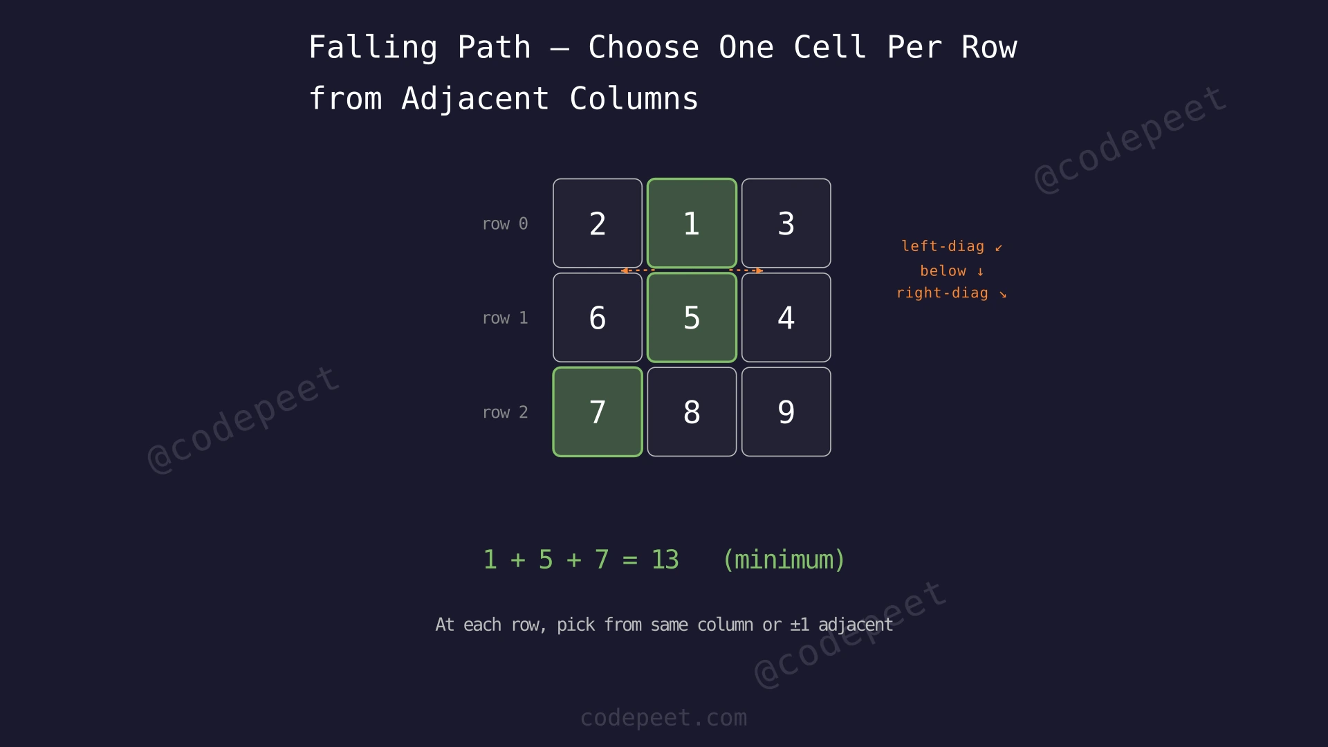
A falling path starts at any element in the first row and proceeds to the last row by choosing one element from each row. The next element you pick must be in a column that is directly below or diagonally left/right of the current column. Formally, from position (row, col), the next position can be:
(row + 1, col - 1)— diagonally left(row + 1, col)— directly below(row + 1, col + 1)— diagonally right
The sum of a falling path is the total of all elements visited along the path. Your task is to find the falling path that gives the smallest possible sum.
Examples
Example 1
Input: matrix = [[2,1,3],[6,5,4],[7,8,9]]
Output: 13
Explanation: There are two falling paths that achieve the minimum sum of 13:
- Path 1: 1 → 5 → 7 (columns 1 → 1 → 0), sum = 1 + 5 + 7 = 13
- Path 2: 1 → 4 → 8 (columns 1 → 2 → 1), sum = 1 + 4 + 8 = 13
Both paths start at row 0, column 1 (value 1), which is the smallest value in the first row. No falling path through this matrix has a sum smaller than 13.
Example 2
Input: matrix = [[-19,57],[-40,-5]]
Output: -59
Explanation: There are two possible falling paths starting from row 0:
- Start at (-19): go to (-40) → sum = -19 + (-40) = -59
- Start at (-19): go to (-5) → sum = -19 + (-5) = -24
- Start at (57): go to (-40) → sum = 57 + (-40) = 17
- Start at (57): go to (-5) → sum = 57 + (-5) = 52
The minimum sum is -59 from path -19 → -40. Note that negative values make the sum smaller, so we prefer them.
Example 3
Input: matrix = [[5]]
Output: 5
Explanation: With a 1×1 matrix, the only falling path is the single element itself. The minimum sum is simply 5.
Constraints
- n == matrix.length == matrix[i].length
- 1 ≤ n ≤ 100
- -100 ≤ matrix[i][j] ≤ 100
Editorial
Brute Force
Intuition
The most straightforward approach is to try every possible falling path and keep track of the minimum sum we find.
Imagine standing at the top of a mountain with multiple trails leading down. At each level (row), the trail can fork left, straight, or right. To find the easiest trail (minimum total cost), you could physically walk every single trail, measure the effort for each, and then compare all of them.
We can implement this using recursion. For each cell in the first row, we start a recursive exploration: from the current cell, try all valid moves to the next row (up to 3 choices), recursively find the minimum path sum from each of those cells onward, and add the current cell's value.
The recursion naturally explores every possible path. The base case is reaching the last row — there are no more rows to descend into, so we just return the cell's value.
Step-by-Step Explanation
Let's trace through with matrix = [[2,1,3],[6,5,4],[7,8,9]]:
Step 1: We try starting from every cell in row 0: (0,0)=2, (0,1)=1, (0,2)=3.
Step 2: Start from (0,1)=1 (we'll trace this starting point in detail). From (0,1), we can move to (1,0)=6, (1,1)=5, or (1,2)=4.
Step 3: Explore path (0,1)→(1,0)=6, sum so far = 7.
- From (1,0), move to (2,0)=7: path 1→6→7 = 14 (complete path)
- From (1,0), move to (2,1)=8: path 1→6→8 = 15 (complete path)
- Best from (1,0): 14
Step 4: Explore path (0,1)→(1,1)=5, sum so far = 6.
- From (1,1), move to (2,0)=7: path 1→5→7 = 13 (complete)
- From (1,1), move to (2,1)=8: path 1→5→8 = 14 (complete)
- From (1,1), move to (2,2)=9: path 1→5→9 = 15 (complete)
- Best from (1,1): 13
Step 5: Explore path (0,1)→(1,2)=4, sum so far = 5.
- From (1,2), move to (2,1)=8: path 1→4→8 = 13 (complete)
- From (1,2), move to (2,2)=9: path 1→4→9 = 14 (complete)
- Best from (1,2): 13
Step 6: Best from starting cell (0,1): min(14, 13, 13) = 13.
Step 7: Similarly explore from (0,0)=2 and (0,2)=3 (best from (0,0) is 14, best from (0,2) is 15).
Step 8: Global minimum = min(14, 13, 15) = 13.
We explored a total of 13 complete paths across all starting cells.
Brute Force — Exploring All Falling Paths — Watch how the brute force approach recursively explores every possible falling path from a starting cell, backtracking after each complete path to try the next branch.
Algorithm
- For each cell in the first row (column 0 to n-1), start a recursive search.
- Define a recursive function
dfs(row, col)that returns the minimum falling path sum starting from cell (row, col):
a. Base case: If col is out of bounds (col < 0 or col ≥ n), return infinity (invalid path).
b. Base case: If row == n-1 (last row), return matrix[row][col] (no more rows to descend).
c. Recursive case: Return matrix[row][col] + min(dfs(row+1, col-1), dfs(row+1, col), dfs(row+1, col+1)). - The answer is the minimum of
dfs(0, col)for all col from 0 to n-1.
Code
#include <vector>
#include <algorithm>
#include <climits>
using namespace std;

class Solution {
public:
    int minFallingPathSum(
        vector<vector<int>>& matrix) {
        int n = matrix.size();
        int result = INT_MAX;
        for (int col = 0; col < n; col++) {
            result = min(result,
                dfs(matrix, 0, col, n));
        }
        return result;
    }

private:
    int dfs(vector<vector<int>>& matrix,
        int row, int col, int n) {
        // Out of bounds
        if (col < 0 || col >= n)
            return INT_MAX;
        // Reached last row
        if (row == n - 1)
            return matrix[row][col];

        int down = dfs(matrix, row+1, col, n);
        int left = dfs(matrix, row+1, col-1, n);
        int right = dfs(matrix, row+1, col+1, n);

        return matrix[row][col]
            + min({down, left, right});
    }
};
class Solution:
def minFallingPathSum(
self, matrix: list[list[int]]
) -> int:
n = len(matrix)
def dfs(row: int, col: int) -> int:
# Out of bounds
if col < 0 or col >= n:
return float('inf')
# Reached last row
if row == n - 1:
return matrix[row][col]
down = dfs(row + 1, col)
left = dfs(row + 1, col - 1)
right = dfs(row + 1, col + 1)
return matrix[row][col] + min(
down, left, right
)
return min(
dfs(0, col) for col in range(n)
)class Solution {
public int minFallingPathSum(
int[][] matrix) {
int n = matrix.length;
int result = Integer.MAX_VALUE;
for (int col = 0; col < n; col++) {
result = Math.min(result,
dfs(matrix, 0, col, n));
}
return result;
}
private int dfs(int[][] matrix,
int row, int col, int n) {
if (col < 0 || col >= n)
return Integer.MAX_VALUE;
if (row == n - 1)
return matrix[row][col];
int down = dfs(matrix, row+1, col, n);
int left = dfs(matrix, row+1, col-1, n);
int right = dfs(matrix, row+1, col+1, n);
return matrix[row][col]
+ Math.min(down,
Math.min(left, right));
}
}Complexity Analysis
Time Complexity: O(n × 3^n)
For each of the n starting cells in row 0, the recursion branches into up to 3 choices at every row. With n rows, this creates up to 3^(n-1) paths per starting cell. Total: n × 3^(n-1) = O(n × 3^n).
For a 100×100 matrix, 3^100 ≈ 5 × 10^47 — astronomically large. This approach is hopelessly slow for any non-trivial input.
Space Complexity: O(n)
The recursion depth is n (one call per row), so the call stack uses O(n) space.
Why This Approach Is Not Efficient
The brute force has exponential time complexity O(n × 3^n). Even for a modest 20×20 matrix, 3^20 ≈ 3.5 billion — far too slow.
The fundamental flaw is redundant computation. Many recursive calls compute the same subproblem repeatedly. For example, the call dfs(1, 1) (minimum path from cell (1,1) to the bottom) might be triggered from dfs(0, 0), dfs(0, 1), and dfs(0, 2) — the same work done three times.
In general, there are only n × n = n² unique subproblems (one per cell), but the brute force explores 3^n paths — an exponential number of calls to solve a polynomial number of subproblems.
Key Insight: Since the same cell's result is needed by multiple parent cells, we can store (cache) it after the first computation. This is dynamic programming — solve each subproblem once and reuse the result. This collapses the exponential 3^n into just n² computations.
Better Approach - 2D Dynamic Programming (Tabulation)
Intuition
Instead of recursively exploring from top to bottom and repeating work, we can build the solution bottom-up using a 2D DP table.
Define dp[i][j] as the minimum falling path sum that ends at cell (i, j). For the first row, dp[0][j] = matrix[0][j] (the path has only one cell). For subsequent rows, the value at dp[i][j] comes from the best (minimum) of the three cells above it in the previous row, plus the current cell's value:
dp[i][j] = matrix[i][j] + min(dp[i-1][j-1], dp[i-1][j], dp[i-1][j+1])
(with boundary checks for the first and last columns)
Think of it like filling a spreadsheet row by row. Each cell's value depends only on three cells in the row above. Once we fill the entire table, the answer is the smallest value in the last row — that represents the minimum path sum ending at any column in the final row.
This eliminates all redundant computation: each of the n² cells is computed exactly once.
Step-by-Step Explanation
Let's trace with matrix = [[2,1,3],[6,5,4],[7,8,9]]:
Step 1: Create a 3×3 DP table. Fill base case — first row copies directly from matrix:
- dp[0][0] = 2, dp[0][1] = 1, dp[0][2] = 3
Step 2: Fill row 1, column 0:
- dp[1][0] = matrix[1][0] + min(dp[0][0], dp[0][1]) = 6 + min(2, 1) = 6 + 1 = 7
- (Column 0 has no left-diagonal neighbor, so we only check above and above-right)
Step 3: Fill row 1, column 1:
- dp[1][1] = matrix[1][1] + min(dp[0][0], dp[0][1], dp[0][2]) = 5 + min(2, 1, 3) = 5 + 1 = 6
- (Middle columns check all three neighbors above)
Step 4: Fill row 1, column 2:
- dp[1][2] = matrix[1][2] + min(dp[0][1], dp[0][2]) = 4 + min(1, 3) = 4 + 1 = 5
- (Last column has no right-diagonal neighbor)
Step 5: Fill row 2, column 0:
- dp[2][0] = matrix[2][0] + min(dp[1][0], dp[1][1]) = 7 + min(7, 6) = 7 + 6 = 13
Step 6: Fill row 2, column 1:
- dp[2][1] = matrix[2][1] + min(dp[1][0], dp[1][1], dp[1][2]) = 8 + min(7, 6, 5) = 8 + 5 = 13
Step 7: Fill row 2, column 2:
- dp[2][2] = matrix[2][2] + min(dp[1][1], dp[1][2]) = 9 + min(6, 5) = 9 + 5 = 14
Step 8: Answer = min(dp[2][0], dp[2][1], dp[2][2]) = min(13, 13, 14) = 13.
2D DP Table — Filling Row by Row — Watch how each cell in the DP table is computed from the minimum of up to three cells in the previous row, building the solution from top to bottom.
Algorithm
- Create a 2D array
dpof size n × n. - Base case: Copy the first row of the matrix into
dp[0]. - Fill row by row: For each row i from 1 to n-1:
- For each column j from 0 to n-1:
- Find the minimum value among
dp[i-1][j-1],dp[i-1][j],dp[i-1][j+1](with boundary checks). - Set
dp[i][j] = matrix[i][j] + min_above.
- Find the minimum value among
- For each column j from 0 to n-1:
- Answer: Return the minimum value in the last row
dp[n-1].
Code
#include <vector>
#include <algorithm>
using namespace std;

class Solution {
public:
    int minFallingPathSum(
        vector<vector<int>>& matrix) {
        int n = matrix.size();
        vector<vector<int>> dp(n,
            vector<int>(n));

        // Base case: first row
        for (int j = 0; j < n; j++)
            dp[0][j] = matrix[0][j];

        // Fill row by row
        for (int i = 1; i < n; i++) {
            for (int j = 0; j < n; j++) {
                int best = dp[i-1][j];
                if (j > 0)
                    best = min(best,
                        dp[i-1][j-1]);
                if (j + 1 < n)
                    best = min(best,
                        dp[i-1][j+1]);
                dp[i][j] = matrix[i][j] + best;
            }
        }

        return *min_element(
            dp[n-1].begin(), dp[n-1].end());
    }
};
class Solution:
def minFallingPathSum(
self, matrix: list[list[int]]
) -> int:
n = len(matrix)
dp = [[0] * n for _ in range(n)]
# Base case: first row
for j in range(n):
dp[0][j] = matrix[0][j]
# Fill row by row
for i in range(1, n):
for j in range(n):
best = dp[i-1][j]
if j > 0:
best = min(best,
dp[i-1][j-1])
if j + 1 < n:
best = min(best,
dp[i-1][j+1])
dp[i][j] = matrix[i][j] + best
return min(dp[n-1])class Solution {
public int minFallingPathSum(
int[][] matrix) {
int n = matrix.length;
int[][] dp = new int[n][n];
// Base case: first row
for (int j = 0; j < n; j++)
dp[0][j] = matrix[0][j];
// Fill row by row
for (int i = 1; i < n; i++) {
for (int j = 0; j < n; j++) {
int best = dp[i-1][j];
if (j > 0)
best = Math.min(best,
dp[i-1][j-1]);
if (j + 1 < n)
best = Math.min(best,
dp[i-1][j+1]);
dp[i][j] = matrix[i][j] + best;
}
}
int result = dp[n-1][0];
for (int j = 1; j < n; j++)
result = Math.min(result,
dp[n-1][j]);
return result;
}
}Complexity Analysis
Time Complexity: O(n²)
We iterate through each of the n² cells exactly once. For each cell, we look at up to 3 values in the previous row (constant work). Total: n² × O(1) = O(n²).
For n = 100, this is just 10,000 operations — practically instant compared to the brute force's 3^100 ≈ 5 × 10^47.
Space Complexity: O(n²)
We store the entire n × n DP table. For n = 100, this is 10,000 integers — completely fine for memory.
Why This Approach Is Not Efficient
The 2D DP approach has optimal O(n²) time complexity — we cannot do better since we must examine each cell at least once. However, its space complexity O(n²) can be improved.
Notice that when computing row i, we only need row i-1. Rows i-2, i-3, etc. are never accessed again. Yet the 2D DP table stores all n rows permanently.
This is a common DP pattern: when the recurrence depends only on the immediately previous row, we can compress the 2D table into two 1D arrays (one for the previous row and one for the current row being computed). After processing each row, we swap them.
This reduces space from O(n²) to O(n) while keeping the same O(n²) time.
Optimal Approach - Space-Optimized Dynamic Programming
Intuition
The space-optimized approach exploits a key observation: we only need the previous row's DP values to compute the current row. There is no need to keep the entire 2D table.
Imagine a factory assembly line. At each station (row), workers only need the output from the immediately preceding station. They don't need to see outputs from two or three stations back. So instead of storing results from every station, we keep only a single shelf of results (one 1D array) and overwrite it as each new station finishes.
Concretely, we maintain an array prev of size n holding the minimum path sums for the previous row. For each new row, we compute a fresh array curr using prev, then replace prev with curr for the next iteration. After processing all rows, the answer is min(prev).
The time complexity remains O(n²), but space drops from O(n²) to O(n) — a significant improvement for large n.
Step-by-Step Explanation
Let's trace with matrix = [[2,1,3],[6,5,4],[7,8,9]]:
Step 1: Initialize prev = [2, 1, 3] (copy first row of matrix).
Step 2: Process row 1. Create curr = [-, -, -].
- curr[0] = matrix[1][0] + min(prev[0], prev[1]) = 6 + min(2, 1) = 7
- curr[1] = matrix[1][1] + min(prev[0], prev[1], prev[2]) = 5 + min(2, 1, 3) = 6
- curr[2] = matrix[1][2] + min(prev[1], prev[2]) = 4 + min(1, 3) = 5
Step 3: Swap: prev = [7, 6, 5]. Discard old prev — it's no longer needed.
Step 4: Process row 2. Create curr = [-, -, -].
- curr[0] = matrix[2][0] + min(prev[0], prev[1]) = 7 + min(7, 6) = 13
- curr[1] = matrix[2][1] + min(prev[0], prev[1], prev[2]) = 8 + min(7, 6, 5) = 13
- curr[2] = matrix[2][2] + min(prev[1], prev[2]) = 9 + min(6, 5) = 14
Step 5: Swap: prev = [13, 13, 14]. All rows processed.
Step 6: Answer = min(prev) = min(13, 13, 14) = 13.
Space-Optimized DP — Rolling Two Arrays — Watch how we maintain just two arrays (prev and curr) instead of a full 2D table. After each row, curr becomes prev and the old data is discarded.
Algorithm
- Initialize
prevas a copy of the first row of the matrix. - For each row
ifrom 1 to n-1:
a. Create a new arraycurrof size n.
b. For each columnjfrom 0 to n-1:- Compute
best= minimum of prev[j-1], prev[j], prev[j+1] (with boundary checks). - Set
curr[j] = matrix[i][j] + best.
c. Setprev = curr(discard old prev).
- Compute
- Return
min(prev)— the minimum value in the last processed row.
Code
#include <vector>
#include <algorithm>
using namespace std;

class Solution {
public:
    int minFallingPathSum(
        vector<vector<int>>& matrix) {
        int n = matrix.size();
        // Start with first row
        vector<int> prev(matrix[0].begin(),
            matrix[0].end());

        for (int i = 1; i < n; i++) {
            vector<int> curr(n);
            for (int j = 0; j < n; j++) {
                int best = prev[j];
                if (j > 0)
                    best = min(best, prev[j-1]);
                if (j + 1 < n)
                    best = min(best, prev[j+1]);
                curr[j] = matrix[i][j] + best;
            }
            prev = curr;
        }

        return *min_element(
            prev.begin(), prev.end());
    }
};
class Solution:
def minFallingPathSum(
self, matrix: list[list[int]]
) -> int:
n = len(matrix)
prev = matrix[0][:] # Copy first row
for i in range(1, n):
curr = [0] * n
for j in range(n):
best = prev[j]
if j > 0:
best = min(best, prev[j-1])
if j + 1 < n:
best = min(best, prev[j+1])
curr[j] = matrix[i][j] + best
prev = curr
return min(prev)class Solution {
public int minFallingPathSum(
int[][] matrix) {
int n = matrix.length;
int[] prev = new int[n];
// Copy first row
for (int j = 0; j < n; j++)
prev[j] = matrix[0][j];
for (int i = 1; i < n; i++) {
int[] curr = new int[n];
for (int j = 0; j < n; j++) {
int best = prev[j];
if (j > 0)
best = Math.min(best,
prev[j-1]);
if (j + 1 < n)
best = Math.min(best,
prev[j+1]);
curr[j] = matrix[i][j] + best;
}
prev = curr;
}
int result = prev[0];
for (int j = 1; j < n; j++)
result = Math.min(result, prev[j]);
return result;
}
}Complexity Analysis
Time Complexity: O(n²)
Same as the 2D DP approach. We process each of the n² cells exactly once, with O(1) work per cell (comparing up to 3 values from the previous row). The space optimization does not affect time complexity.
Space Complexity: O(n)
We maintain only two arrays of size n: prev and curr. After each row, curr replaces prev and the old array is freed. This is a factor-of-n improvement over the O(n²) space of the 2D DP table.
For n = 100, we use just 200 integers of storage instead of 10,000 — a 50× reduction.