Flood Fill
Description
You are given an image represented by an m × n grid of integers called image, where image[i][j] represents the pixel value (color) at row i and column j. You are also given three integers: sr (starting row), sc (starting column), and color (the new color to apply).
Your task is to perform a flood fill starting from the pixel image[sr][sc]:
- Change the color of the starting pixel to
color. - For every pixel that is directly adjacent (shares a side — up, down, left, or right, NOT diagonal) to the starting pixel and has the same original color as the starting pixel, change its color to
coloras well. - Continue this process recursively for all newly colored pixels — check their neighbors, and color those that match the original color.
- Stop when no more adjacent pixels with the original color can be found.
Return the modified image after performing the flood fill.
Key insight: This is essentially asking you to find all pixels that are connected to the starting pixel through a chain of same-colored, 4-directionally adjacent pixels, and change all of them to the new color. Pixels that have the original color but are separated by differently-colored pixels remain unchanged.
Examples
Example 1
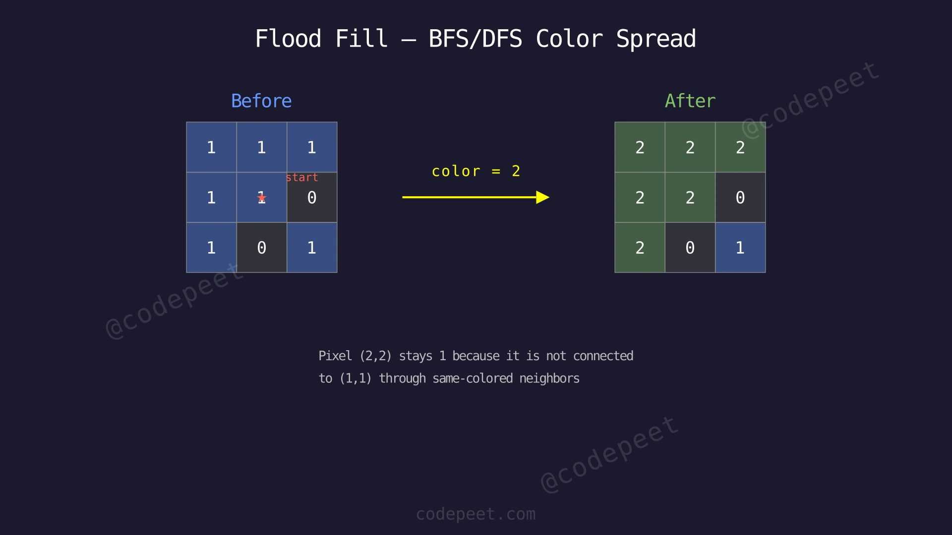
Input: image = [[1,1,1],[1,1,0],[1,0,1]], sr = 1, sc = 1, color = 2
Output: [[2,2,2],[2,2,0],[2,0,1]]
Explanation: Starting from the center pixel (1,1) which has color 1, we change it to 2. Then we check its four neighbors:
- Up (0,1) = 1 → same as original, change to 2
- Down (2,1) = 0 → different color, skip
- Left (1,0) = 1 → same as original, change to 2
- Right (1,2) = 0 → different color, skip
We continue this process for each newly colored pixel until all connected pixels are updated. The pixel at (2,2) has value 1, but it is NOT reachable from (1,1) through same-colored neighbors because cells (1,2)=0 and (2,1)=0 block the path. So it stays as 1.
Example 2
Input: image = [[0,0,0],[0,0,0]], sr = 0, sc = 0, color = 0
Output: [[0,0,0],[0,0,0]]
Explanation: The starting pixel at (0,0) already has color 0, which is the same as the target color. Since old color equals new color, no changes need to be made. This is an important edge case — if we do not handle it, we might enter an infinite loop because every neighbor we color would still match the 'old' color.
Example 3
Input: image = [[1,1,1,0],[0,1,1,1],[1,0,1,1]], sr = 1, sc = 2, color = 3
Output: [[3,3,3,0],[0,3,3,3],[1,0,3,3]]
Explanation: Starting from pixel (1,2) with color 1, we flood fill outward. The connected region includes (0,0), (0,1), (0,2), (1,1), (1,2), (1,3), (2,2), (2,3) — all reachable from (1,2) through same-colored neighbors. Pixel (2,0) has color 1 but is isolated from the starting pixel by the 0-valued cells at (1,0) and (2,1), so it remains 1.
Constraints
- m == image.length
- n == image[i].length
- 1 ≤ m, n ≤ 50
- 0 ≤ image[i][j], color < 2^16
- 0 ≤ sr < m
- 0 ≤ sc < n
- The image grid is non-empty
- The starting pixel (sr, sc) is always within bounds
Editorial
Brute Force
Intuition
The most natural way to think about flood fill is like pouring paint from a bucket. You start at one pixel, pour the new color on it, then the paint "spreads" to all neighboring pixels that share the original color.
Imagine you are painting a wall and you dip your roller in green paint and place it at one spot on a blue wall. The green paint naturally flows to all connected blue areas, but it cannot cross boundaries of other colors (red trim, white borders, etc.).
This "spreading" behavior maps perfectly to Depth-First Search (DFS). We start at the given pixel, change its color, then recursively visit each of its four neighbors. If a neighbor has the same original color, we change it and repeat. If a neighbor is out of bounds, has a different color, or has already been changed, we stop.
The recursion naturally handles the "spreading" — each call handles one pixel and delegates its neighbors to further recursive calls. When all connected same-colored pixels have been visited, the recursion unwinds and we are done.
Critical edge case: If the starting pixel's color is ALREADY equal to the new color, we must return immediately without doing anything. Otherwise, since we use oldColor != image[r][c] as our stopping condition, every neighbor would still match oldColor after being "colored" (because old and new are the same), leading to infinite recursion.
Step-by-Step Explanation
Let's trace through with image = [[1,1,1],[1,1,0],[1,0,1]], sr=1, sc=1, color=2.
oldColor = image[1][1] = 1, newColor = 2.
Step 1: Start DFS at (1,1). Its value is 1 (matches oldColor). Change (1,1) from 1 → 2.
- Grid: [[1,1,1],[1,2,0],[1,0,1]]
Step 2: Recurse up to (0,1). Its value is 1 (matches oldColor). Change (0,1) from 1 → 2.
- Grid: [[1,2,1],[1,2,0],[1,0,1]]
Step 3: From (0,1), recurse left to (0,0). Its value is 1 (matches oldColor). Change (0,0) from 1 → 2.
- Grid: [[2,2,1],[1,2,0],[1,0,1]]
Step 4: From (0,0), recurse down to (1,0). Its value is 1 (matches oldColor). Change (1,0) from 1 → 2.
- Grid: [[2,2,1],[2,2,0],[1,0,1]]
Step 5: From (1,0), recurse down to (2,0). Its value is 1 (matches oldColor). Change (2,0) from 1 → 2.
- Grid: [[2,2,1],[2,2,0],[2,0,1]]
Step 6: From (2,0), check right neighbor (2,1) = 0. Does NOT match oldColor (1). Skip. All other neighbors of (2,0) are out of bounds or already colored. Backtrack.
Step 7: Backtrack to (0,1). Now recurse right to (0,2). Its value is 1 (matches oldColor). Change (0,2) from 1 → 2.
- Grid: [[2,2,2],[2,2,0],[2,0,1]]
Step 8: From (0,2), check down neighbor (1,2) = 0. Does NOT match oldColor. No more valid neighbors from (0,2). Backtrack.
Step 9: Backtrack all the way to (1,1). Check remaining neighbors: down (2,1) = 0 (skip), right (1,2) = 0 (skip). All done.
Step 10: DFS complete. Final grid: [[2,2,2],[2,2,0],[2,0,1]]. The pixel at (2,2) = 1 remains unchanged because it is completely surrounded by 0-valued cells on its path to the start.
Flood Fill — DFS Recursive Exploration — Watch how DFS dives deep from the starting pixel, coloring each connected pixel and backtracking when it hits boundaries or different colors.
Algorithm
- Store the original color of the starting pixel as
oldColor - Edge case check: If
oldColor == newColor, return the image unchanged (prevents infinite recursion) - Call
dfs(image, sr, sc, oldColor, newColor) - In the DFS function:
a. If the current position is out of bounds, return
b. If the current pixel's color is NOToldColor, return
c. Change the current pixel's color tonewColor
d. Recursively call DFS on all four neighbors: up, down, left, right - Return the modified image
Code
class Solution {
public:
    vector<vector<int>> floodFill(vector<vector<int>>& image, int sr, int sc, int color) {
        int oldColor = image[sr][sc];
        if (oldColor == color) return image;
        dfs(image, sr, sc, oldColor, color);
        return image;
    }

private:
    void dfs(vector<vector<int>>& image, int r, int c, int oldColor, int newColor) {
        if (r < 0 || r >= image.size() || c < 0 || c >= image[0].size()) return;
        if (image[r][c] != oldColor) return;

        image[r][c] = newColor;
        dfs(image, r - 1, c, oldColor, newColor);
        dfs(image, r + 1, c, oldColor, newColor);
        dfs(image, r, c - 1, oldColor, newColor);
        dfs(image, r, c + 1, oldColor, newColor);
    }
};
class Solution:
def floodFill(self, image: list[list[int]], sr: int, sc: int, color: int) -> list[list[int]]:
old_color = image[sr][sc]
if old_color == color:
return image
self._dfs(image, sr, sc, old_color, color)
return image
def _dfs(self, image, r, c, old_color, new_color):
if r < 0 or r >= len(image) or c < 0 or c >= len(image[0]):
return
if image[r][c] != old_color:
return
image[r][c] = new_color
self._dfs(image, r - 1, c, old_color, new_color)
self._dfs(image, r + 1, c, old_color, new_color)
self._dfs(image, r, c - 1, old_color, new_color)
self._dfs(image, r, c + 1, old_color, new_color)class Solution {
public int[][] floodFill(int[][] image, int sr, int sc, int color) {
int oldColor = image[sr][sc];
if (oldColor == color) return image;
dfs(image, sr, sc, oldColor, color);
return image;
}
private void dfs(int[][] image, int r, int c, int oldColor, int newColor) {
if (r < 0 || r >= image.length || c < 0 || c >= image[0].length) return;
if (image[r][c] != oldColor) return;
image[r][c] = newColor;
dfs(image, r - 1, c, oldColor, newColor);
dfs(image, r + 1, c, oldColor, newColor);
dfs(image, r, c - 1, oldColor, newColor);
dfs(image, r, c + 1, oldColor, newColor);
}
}Complexity Analysis
Time Complexity: O(m × n)
In the worst case, every pixel in the grid has the same color as the starting pixel, meaning DFS visits all m × n pixels. Each pixel is visited at most once because once we change its color from oldColor to newColor, subsequent DFS calls that reach it will see image[r][c] != oldColor and return immediately. So the total work is proportional to the number of pixels.
Space Complexity: O(m × n)
The recursion stack can grow as deep as the number of pixels in the connected component. In the worst case (e.g., a single long winding path covering the entire grid), the recursion depth reaches m × n. Each recursive call uses O(1) stack space, so total space is O(m × n).
For this problem's constraints (m, n ≤ 50), the maximum recursion depth is 2500, which is manageable. However, for larger grids (e.g., 1000 × 1000), the recursion depth of up to 10^6 could cause a stack overflow in languages with limited default stack sizes (Python's default recursion limit is 1000, Java's default thread stack is ~512KB).
Why This Approach Is Not Efficient
While the DFS approach has the same asymptotic time complexity as BFS — O(m × n) — it has practical disadvantages:
-
Stack overflow risk: The recursive DFS uses the system call stack, which has a limited size. For a 1000×1000 grid where all pixels share one color, the recursion depth can reach 10^6, far exceeding most language defaults. Python's default limit is 1000 recursive calls. Java and C++ have fixed stack sizes that can overflow for deep recursion.
-
Function call overhead: Each recursive call incurs overhead for creating a new stack frame (saving local variables, return address, etc.). For millions of pixels, this overhead adds up compared to an iterative approach.
-
No traversal order control: DFS explores deeply in one direction before backtracking. This means the "paint" fills in a somewhat erratic zigzag pattern rather than a smooth outward spread. While the final result is identical, BFS gives a more natural and predictable "wave-like" fill pattern.
-
Harder to adapt: If we later wanted to limit the fill to pixels within a certain distance from the start, BFS's level-by-level nature makes this trivial, while DFS would require additional tracking.
An iterative BFS approach eliminates the stack overflow risk by using an explicit queue, and provides a more intuitive exploration order.
Optimal Approach - BFS (Iterative)
Intuition
Instead of diving deep into one direction before backtracking (DFS), we can spread the paint outward like a ripple in a pond. Drop a stone at the starting pixel, and the color change radiates outward one layer at a time — first the starting pixel, then its immediate neighbors, then their neighbors, and so on.
This ripple-like behavior is exactly what Breadth-First Search (BFS) provides. We use a queue to process pixels in the order they are discovered:
- Start by putting the starting pixel in the queue and changing its color
- Repeatedly dequeue a pixel, check its four neighbors
- If a neighbor has the original color, change it and enqueue it
- Continue until the queue is empty
Since BFS uses an explicit queue rather than the system call stack, there is no risk of stack overflow regardless of grid size. The queue is allocated on the heap, which can typically handle much larger sizes.
The time and space complexity remain O(m × n) — the same as DFS. The improvement is entirely practical: no recursion depth limit, predictable memory usage, and a more intuitive wave-like fill pattern.
Step-by-Step Explanation
Let's trace BFS with the same example: image = [[1,1,1],[1,1,0],[1,0,1]], sr=1, sc=1, color=2.
oldColor = 1, newColor = 2.
Step 1: Change starting pixel (1,1) to 2 and enqueue it.
- Grid: [[1,1,1],[1,2,0],[1,0,1]]
- Queue: [(1,1)]
Step 2: Dequeue (1,1). Check its four neighbors:
- Up (0,1) = 1 → matches oldColor. Change to 2, enqueue.
- Down (2,1) = 0 → different color, skip.
- Left (1,0) = 1 → matches oldColor. Change to 2, enqueue.
- Right (1,2) = 0 → different color, skip.
- Grid: [[1,2,1],[2,2,0],[1,0,1]]
- Queue: [(0,1), (1,0)]
Step 3: Dequeue (0,1). Check neighbors:
- Up (-1,1) → out of bounds, skip.
- Down (1,1) = 2 → already changed, skip.
- Left (0,0) = 1 → matches oldColor. Change to 2, enqueue.
- Right (0,2) = 1 → matches oldColor. Change to 2, enqueue.
- Grid: [[2,2,2],[2,2,0],[1,0,1]]
- Queue: [(1,0), (0,0), (0,2)]
Step 4: Dequeue (1,0). Check neighbors:
- Up (0,0) = 2 → already changed, skip.
- Down (2,0) = 1 → matches oldColor. Change to 2, enqueue.
- Left (1,-1) → out of bounds, skip.
- Right (1,1) = 2 → already changed, skip.
- Grid: [[2,2,2],[2,2,0],[2,0,1]]
- Queue: [(0,0), (0,2), (2,0)]
Step 5: Dequeue (0,0). All neighbors are either out of bounds or already color 2. Nothing to do.
- Queue: [(0,2), (2,0)]
Step 6: Dequeue (0,2). Down (1,2) = 0, skip. All other neighbors out of bounds or already 2.
- Queue: [(2,0)]
Step 7: Dequeue (2,0). Right (2,1) = 0, skip. All other neighbors out of bounds or already 2.
- Queue: []
Step 8: Queue is empty. BFS complete. Final grid: [[2,2,2],[2,2,0],[2,0,1]].
Flood Fill — BFS Wave-Like Expansion — Watch how BFS spreads the new color outward in waves, processing all pixels at distance 1 before distance 2, like ripples in a pond.
Algorithm
- Store the original color:
oldColor = image[sr][sc] - Edge case check: If
oldColor == newColor, return the image unchanged - Create a queue and add the starting pixel
(sr, sc) - Change
image[sr][sc]tonewColor - While the queue is not empty:
a. Dequeue a pixel(r, c)
b. For each of the 4 directions (up, down, left, right):- Calculate the neighbor position
(nr, nc) - If
(nr, nc)is within bounds ANDimage[nr][nc] == oldColor:- Change
image[nr][nc]tonewColor - Enqueue
(nr, nc)
- Change
- Calculate the neighbor position
- Return the modified image
Code
class Solution {
public:
    vector<vector<int>> floodFill(vector<vector<int>>& image, int sr, int sc, int color) {
        int oldColor = image[sr][sc];
        if (oldColor == color) return image;

        int m = image.size(), n = image[0].size();
        int dirs[4][2] = {{-1, 0}, {1, 0}, {0, -1}, {0, 1}};

        queue<pair<int, int>> q;
        q.push({sr, sc});
        image[sr][sc] = color;

        while (!q.empty()) {
            auto [r, c] = q.front();
            q.pop();

            for (auto& d : dirs) {
                int nr = r + d[0], nc = c + d[1];
                if (nr >= 0 && nr < m && nc >= 0 && nc < n
                    && image[nr][nc] == oldColor) {
                    image[nr][nc] = color;
                    q.push({nr, nc});
                }
            }
        }

        return image;
    }
};
from collections import deque
class Solution:
def floodFill(self, image: list[list[int]], sr: int, sc: int, color: int) -> list[list[int]]:
old_color = image[sr][sc]
if old_color == color:
return image
m, n = len(image), len(image[0])
directions = [(-1, 0), (1, 0), (0, -1), (0, 1)]
queue = deque([(sr, sc)])
image[sr][sc] = color
while queue:
r, c = queue.popleft()
for dr, dc in directions:
nr, nc = r + dr, c + dc
if 0 <= nr < m and 0 <= nc < n and image[nr][nc] == old_color:
image[nr][nc] = color
queue.append((nr, nc))
return imageclass Solution {
public int[][] floodFill(int[][] image, int sr, int sc, int color) {
int oldColor = image[sr][sc];
if (oldColor == color) return image;
int m = image.length, n = image[0].length;
int[][] dirs = {{-1, 0}, {1, 0}, {0, -1}, {0, 1}};
Queue<int[]> queue = new LinkedList<>();
queue.add(new int[]{sr, sc});
image[sr][sc] = color;
while (!queue.isEmpty()) {
int[] pixel = queue.poll();
int r = pixel[0], c = pixel[1];
for (int[] d : dirs) {
int nr = r + d[0], nc = c + d[1];
if (nr >= 0 && nr < m && nc >= 0 && nc < n
&& image[nr][nc] == oldColor) {
image[nr][nc] = color;
queue.add(new int[]{nr, nc});
}
}
}
return image;
}
}Complexity Analysis
Time Complexity: O(m × n)
Each pixel is enqueued and dequeued at most once, because we change its color immediately upon enqueuing (so it will never match oldColor again when checked by another neighbor). For each pixel, we check 4 neighbors in O(1) time. Total operations: at most m × n dequeues × 4 neighbor checks each = O(4 × m × n) = O(m × n).
Space Complexity: O(m × n)
The queue can hold at most all pixels in the grid if the entire image is one connected component of the same color. In practice, the maximum queue size at any point is proportional to the perimeter of the current wave front, which for a square grid is O(min(m, n)). However, the worst case remains O(m × n).
Key advantage over DFS: The space is allocated on the heap (the queue is a dynamically-sized data structure) rather than the system call stack. The heap can typically grow much larger than the call stack. For a 1000×1000 grid, a queue of 10^6 entries uses about 8-16 MB of heap memory — perfectly manageable. In contrast, 10^6 recursive calls would cause a stack overflow in most languages.
Comparison:
| Aspect | DFS (Recursive) | BFS (Iterative) |
|---|---|---|
| Time | O(m × n) | O(m × n) |
| Space | O(m × n) call stack | O(m × n) queue |
| Stack overflow risk | Yes (large grids) | No |
| Fill pattern | Deep zigzag | Wave-like outward |
| Implementation | Simpler (5 lines) | Slightly more code |
| Best for | Small grids, quick coding | Production use, large grids |