Floyd-Warshall Algorithm
Description
You are given a weighted directed graph represented as an n × n adjacency matrix dist[][], where dist[i][j] represents the weight of the direct edge from vertex i to vertex j.
- If there is no direct edge from i to j, then
dist[i][j]is set to 10^8 (representing infinity). - The diagonal entries
dist[i][i]are 0, since the distance from any vertex to itself is zero.
The graph may contain negative weight edges, but it does not contain any negative weight cycles.
Your task is to compute the shortest path distance between every pair of vertices (i, j) in the graph. After running the algorithm, dist[i][j] should hold the shortest distance from vertex i to vertex j, considering all possible intermediate vertices.
This is the all-pairs shortest path problem — unlike single-source algorithms like Dijkstra or Bellman-Ford that find shortest paths from one source, this algorithm finds shortest paths between ALL pairs simultaneously.
Examples
Example 1
Input:
dist[][] = [
  [0,   3,   10^8, 7  ],
  [8,   0,   2,    10^8],
  [5,   10^8, 0,   1  ],
  [2,   10^8, 10^8, 0  ]
]
Output:
[
  [0, 3, 5, 6],
  [5, 0, 2, 3],
  [3, 6, 0, 1],
  [2, 5, 7, 0]
]
Explanation:
- dist[0][2] = 5: The direct edge 0→2 does not exist (10^8), but the path 0→1→2 has weight 3+2 = 5.
- dist[0][3] = 6: The direct edge 0→3 has weight 7, but the path 0→1→2→3 has weight 3+2+1 = 6, which is shorter.
- dist[1][0] = 5: The direct edge 1→0 has weight 8, but the path 1→2→0 has weight 2+5 = 7, and the path 1→2→3→0 has weight 2+1+2 = 5, which is even shorter.
- dist[3][1] = 5: No direct edge 3→1, but the path 3→0→1 has weight 2+3 = 5.
Every cell in the output matrix holds the shortest distance between that pair of vertices, considering all possible intermediate paths.
Example 2
Input:
dist[][] = [
  [0,   4,   10^8],
  [10^8, 0,  -2  ],
  [10^8, 10^8, 0 ]
]
Output:
[
  [0,  4,  2],
  [10^8, 0, -2],
  [10^8, 10^8, 0]
]
Explanation:
- dist[0][2] = 2: No direct edge from 0 to 2, but the path 0→1→2 has weight 4+(-2) = 2. The negative edge from 1 to 2 creates a cheaper route.
- dist[1][0] = 10^8: Vertex 0 is not reachable from vertex 1 (no path exists).
- dist[2][0] = 10^8 and dist[2][1] = 10^8: Vertex 2 has no outgoing edges to reach 0 or 1.
This example demonstrates the algorithm handling negative edge weights correctly.
Constraints
- 1 ≤ n ≤ 500 (where n is the number of vertices)
- -1000 ≤ dist[i][j] ≤ 1000 (for actual edges)
- dist[i][i] = 0 for all i
- dist[i][j] = 10^8 if no direct edge from i to j
- The graph does not contain negative weight cycles
- The graph is directed (dist[i][j] may differ from dist[j][i])
Editorial
Brute Force
Intuition
Since we need the shortest path between every pair of vertices, the most straightforward brute force approach is: run a single-source shortest path algorithm from every vertex.
Imagine you have a map of cities and flight costs between them. To find the cheapest route between every possible pair of cities, you could pick each city as a starting point and then calculate the cheapest route from that city to all others. Repeat this for every city.
Concretely, we run the Bellman-Ford algorithm V times — once with each vertex as the source. Each run of Bellman-Ford computes shortest distances from one source to all other vertices, so V runs give us all-pairs shortest distances.
We use Bellman-Ford (rather than Dijkstra) because the problem allows negative edge weights. Dijkstra does not handle negative edges correctly.
Step-by-Step Explanation
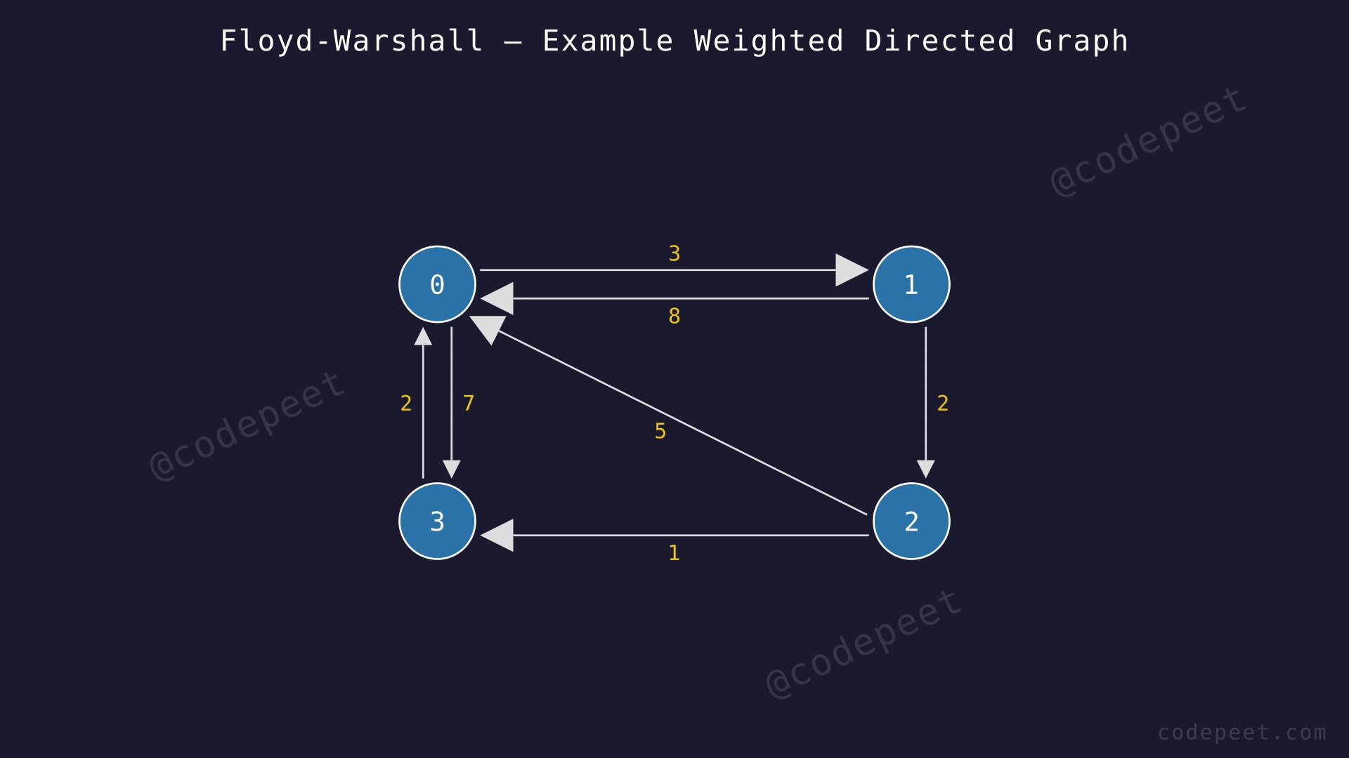
Let's trace through a small example: 4 vertices, adjacency matrix:
dist[][] = [
  [0,   3,   ∞,  7],
  [8,   0,   2,  ∞],
  [5,   ∞,   0,  1],
  [2,   ∞,   ∞,  0]
]
First, convert the matrix to an edge list: (0→1,3), (0→3,7), (1→0,8), (1→2,2), (2→0,5), (2→3,1), (3→0,2).
Step 1: Run Bellman-Ford with source = 0
- Initialize: dist_from_0 = [0, ∞, ∞, ∞]
- Relax edges iteratively:
- After iteration 1: dist_from_0 = [0, 3, ∞, 7] (edges 0→1 and 0→3 relaxed)
- After iteration 2: dist_from_0 = [0, 3, 5, 7] (edge 1→2 relaxed: 3+2=5)
- After iteration 3: dist_from_0 = [0, 3, 5, 6] (edge 2→3 relaxed: 5+1=6)
- Result row 0: [0, 3, 5, 6]
Step 2: Run Bellman-Ford with source = 1
- Initialize: dist_from_1 = [∞, 0, ∞, ∞]
- After relaxation converges: dist_from_1 = [5, 0, 2, 3]
- 1→2 gives dist[2]=2
- 1→2→3 gives dist[3]=3
- 1→2→3→0 gives dist[0]=5 (shortest: 2+1+2=5, better than direct 1→0=8)
- Result row 1: [5, 0, 2, 3]
Step 3: Run Bellman-Ford with source = 2
- Initialize: dist_from_2 = [∞, ∞, 0, ∞]
- After relaxation: dist_from_2 = [3, 6, 0, 1]
- 2→0 gives dist[0]=5, but 2→3→0 gives dist[0]=1+2=3 (shorter!)
- 2→3→0→1 gives dist[1]=1+2+3=6
- Result row 2: [3, 6, 0, 1]
Step 4: Run Bellman-Ford with source = 3
- Initialize: dist_from_3 = [∞, ∞, ∞, 0]
- After relaxation: dist_from_3 = [2, 5, 7, 0]
- 3→0 gives dist[0]=2
- 3→0→1 gives dist[1]=2+3=5
- 3→0→1→2 gives dist[2]=2+3+2=7
- Result row 3: [2, 5, 7, 0]
Step 5: Combine all rows into the result matrix.
Final result:
[0, 3, 5, 6]
[5, 0, 2, 3]
[3, 6, 0, 1]
[2, 5, 7, 0]
Algorithm
- Convert the adjacency matrix to an edge list.
- For each vertex s from 0 to V-1:
a. Run the Bellman-Ford algorithm with source = s.
b. This computes shortest distances from s to all other vertices.
c. Store the results as row s of the output matrix. - Return the complete V × V distance matrix.
Code
#include <vector>
#include <algorithm>
using namespace std;

class Solution {
public:
    void allPairsShortestPath(vector<vector<int>>& dist) {
        int V = dist.size();

        // Build edge list from adjacency matrix
        vector<vector<int>> edges;
        for (int i = 0; i < V; i++) {
            for (int j = 0; j < V; j++) {
                if (i != j && dist[i][j] != (int)1e8) {
                    edges.push_back({i, j, dist[i][j]});
                }
            }
        }

        // Run Bellman-Ford from each vertex
        for (int src = 0; src < V; src++) {
            vector<int> d(V, 1e8);
            d[src] = 0;

            for (int iter = 0; iter < V - 1; iter++) {
                bool updated = false;
                for (auto& e : edges) {
                    int u = e[0], v = e[1], w = e[2];
                    if (d[u] != (int)1e8 && d[u] + w < d[v]) {
                        d[v] = d[u] + w;
                        updated = true;
                    }
                }
                if (!updated) break;
            }

            for (int j = 0; j < V; j++) {
                dist[src][j] = d[j];
            }
        }
    }
};
class Solution:
def allPairsShortestPath(self, dist):
V = len(dist)
# Build edge list from adjacency matrix
edges = []
for i in range(V):
for j in range(V):
if i != j and dist[i][j] != 10**8:
edges.append((i, j, dist[i][j]))
# Run Bellman-Ford from each vertex
for src in range(V):
d = [10**8] * V
d[src] = 0
for _ in range(V - 1):
updated = False
for u, v, w in edges:
if d[u] != 10**8 and d[u] + w < d[v]:
d[v] = d[u] + w
updated = True
if not updated:
break
for j in range(V):
dist[src][j] = d[j]import java.util.*;
class Solution {
public void allPairsShortestPath(int[][] dist) {
int V = dist.length;
// Build edge list from adjacency matrix
List<int[]> edges = new ArrayList<>();
for (int i = 0; i < V; i++) {
for (int j = 0; j < V; j++) {
if (i != j && dist[i][j] != (int)1e8) {
edges.add(new int[]{i, j, dist[i][j]});
}
}
}
// Run Bellman-Ford from each vertex
for (int src = 0; src < V; src++) {
int[] d = new int[V];
Arrays.fill(d, (int)1e8);
d[src] = 0;
for (int iter = 0; iter < V - 1; iter++) {
boolean updated = false;
for (int[] e : edges) {
int u = e[0], v = e[1], w = e[2];
if (d[u] != (int)1e8 && d[u] + w < d[v]) {
d[v] = d[u] + w;
updated = true;
}
}
if (!updated) break;
}
for (int j = 0; j < V; j++) {
dist[src][j] = d[j];
}
}
}
}Complexity Analysis
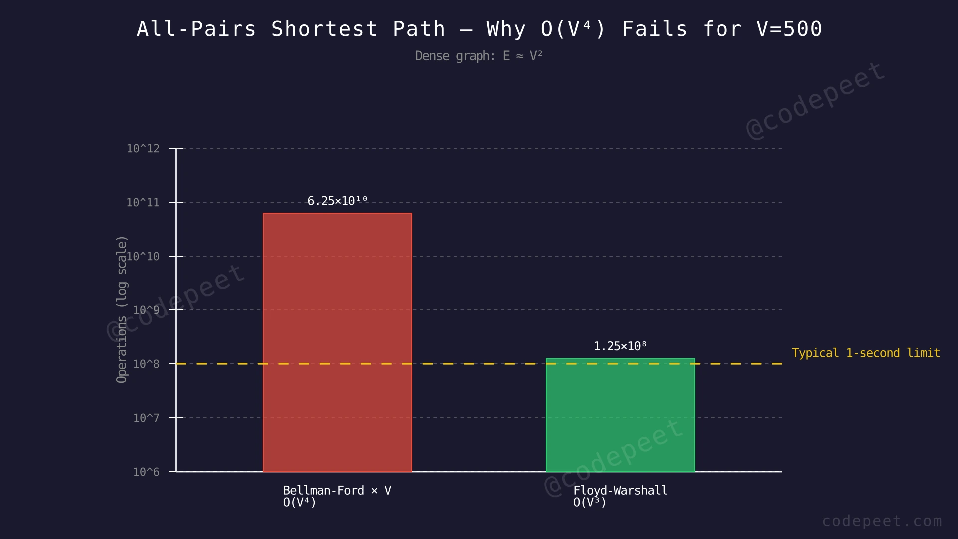
Time Complexity: O(V² × E)
We run Bellman-Ford V times, and each run takes O(V × E) time. The total is O(V × V × E) = O(V² × E).
For a dense graph where E ≈ V², this becomes O(V² × V²) = O(V⁴). With V = 500, that is approximately 500⁴ = 6.25 × 10^10 operations — far too slow for any reasonable time limit.
Even for sparse graphs (E ≈ V), the complexity is O(V³), which is the same as Floyd-Warshall but with worse constant factors.
Space Complexity: O(V + E)
The edge list requires O(E) space (up to O(V²) for dense graphs). Each Bellman-Ford run uses a distance array of size V. We reuse the same temporary array across runs.
Why This Approach Is Not Efficient
The brute force approach of running Bellman-Ford from every vertex has a critical scaling problem:
For dense graphs (the common case for adjacency matrix input), the time complexity is O(V⁴).
With V = 500, this means ~6.25 × 10^10 operations — roughly 100× too slow for a typical 1-second time limit. The problem is that Bellman-Ford processes all edges V-1 times per source, and we have V sources.
The fundamental inefficiency: Each Bellman-Ford run recomputes shortest paths independently, without sharing information across runs. If we already know the shortest path from A to B, this information could help us find the shortest path from C to B — but Bellman-Ford discards it.
The key insight for a better approach:
Instead of thinking "from each source, find paths to all destinations," we can think: "gradually allow more intermediate vertices, and see if any shortest paths improve."
This is the dynamic programming insight behind Floyd-Warshall:
- Start by considering only direct edges (0 intermediate vertices allowed).
- Then allow vertex 0 as an intermediate: does going through vertex 0 create any shorter paths?
- Then allow vertices 0 and 1: does going through vertex 1 create any shorter paths?
- Continue until all vertices are allowed as intermediates.
This approach shares computation across all pairs and runs in exactly O(V³) — a full factor of V faster than the brute force for dense graphs.
Optimal Approach - Floyd-Warshall (Dynamic Programming)
Intuition
The Floyd-Warshall algorithm uses a beautifully simple dynamic programming idea:
Core Question: For each pair of vertices (i, j), does adding vertex k as a potential intermediate stop create a shorter path?
Imagine you are a travel agent. Initially, you only know the direct flight costs between cities. Then, one by one, you "unlock" cities as possible layover points:
- Round 0: Can routing through city 0 make any trip cheaper? For every pair (i, j), check if the cost i→0→j is less than the current cheapest i→j. If so, update.
- Round 1: Can routing through city 1 (possibly also via city 0, which we already considered) make any trip cheaper?
- Round k: Can routing through city k make any trip cheaper?
- After unlocking all cities as intermediates, every shortest path has been discovered.
The mathematical formula at each step is:
dist[i][j] = min(dist[i][j], dist[i][k] + dist[k][j])
This works because of optimal substructure: if the shortest path from i to j goes through k, then the sub-paths i→k and k→j must also be shortest paths. By the time we consider vertex k as an intermediate, all shorter intermediate vertices (0 to k-1) have already been considered, so dist[i][k] and dist[k][j] are already optimal with respect to intermediates 0 through k-1.
The beauty of this approach: three nested loops, no complex data structures, and it handles negative edges correctly.
Step-by-Step Explanation
Let's trace through the 4-vertex example:
Initial distance matrix (direct edges only):
     0    1    2    3
0 [  0,   3,   ∞,   7 ]
1 [  8,   0,   2,   ∞ ]
2 [  5,   ∞,   0,   1 ]
3 [  2,   ∞,   ∞,   0 ]
Step 1: k = 0 (allow vertex 0 as intermediate)
For every pair (i, j), check: is dist[i][0] + dist[0][j] < dist[i][j]?
- (1,3): dist[1][0]+dist[0][3] = 8+7 = 15 vs dist[1][3]=∞. 15 < ∞ → Update dist[1][3] = 15
- (2,1): dist[2][0]+dist[0][1] = 5+3 = 8 vs dist[2][1]=∞. 8 < ∞ → Update dist[2][1] = 8
- (2,3): dist[2][0]+dist[0][3] = 5+7 = 12 vs dist[2][3]=1. 12 > 1 → No update
- (3,1): dist[3][0]+dist[0][1] = 2+3 = 5 vs dist[3][1]=∞. 5 < ∞ → Update dist[3][1] = 5
- (3,3): skip (i=j)
- Other pairs: no improvement
After k=0:
     0    1    2    3
0 [  0,   3,   ∞,   7 ]
1 [  8,   0,   2,  15 ]
2 [  5,   8,   0,   1 ]
3 [  2,   5,   ∞,   0 ]
Step 2: k = 1 (allow vertex 1 as intermediate)
- (0,2): dist[0][1]+dist[1][2] = 3+2 = 5 vs dist[0][2]=∞. 5 < ∞ → Update dist[0][2] = 5
- (0,3): dist[0][1]+dist[1][3] = 3+15 = 18 vs dist[0][3]=7. 18 > 7 → No update
- (2,0): dist[2][1]+dist[1][0] = 8+8 = 16 vs dist[2][0]=5. 16 > 5 → No update
- (3,2): dist[3][1]+dist[1][2] = 5+2 = 7 vs dist[3][2]=∞. 7 < ∞ → Update dist[3][2] = 7
- (3,3): dist[3][1]+dist[1][3] = 5+15 = 20 vs dist[3][3]=0. No update.
After k=1:
     0    1    2    3
0 [  0,   3,   5,   7 ]
1 [  8,   0,   2,  15 ]
2 [  5,   8,   0,   1 ]
3 [  2,   5,   7,   0 ]
Step 3: k = 2 (allow vertex 2 as intermediate)
- (0,3): dist[0][2]+dist[2][3] = 5+1 = 6 vs dist[0][3]=7. 6 < 7 → Update dist[0][3] = 6
- (1,0): dist[1][2]+dist[2][0] = 2+5 = 7 vs dist[1][0]=8. 7 < 8 → Update dist[1][0] = 7
- (1,3): dist[1][2]+dist[2][3] = 2+1 = 3 vs dist[1][3]=15. 3 < 15 → Update dist[1][3] = 3
- (3,0): dist[3][2]+dist[2][0] = 7+5 = 12 vs dist[3][0]=2. 12 > 2 → No update
- (3,3): dist[3][2]+dist[2][3] = 7+1 = 8 vs dist[3][3]=0. No update.
After k=2:
     0    1    2    3
0 [  0,   3,   5,   6 ]
1 [  7,   0,   2,   3 ]
2 [  5,   8,   0,   1 ]
3 [  2,   5,   7,   0 ]
Step 4: k = 3 (allow vertex 3 as intermediate)
- (1,0): dist[1][3]+dist[3][0] = 3+2 = 5 vs dist[1][0]=7. 5 < 7 → Update dist[1][0] = 5
- (2,0): dist[2][3]+dist[3][0] = 1+2 = 3 vs dist[2][0]=5. 3 < 5 → Update dist[2][0] = 3
- (2,1): dist[2][3]+dist[3][1] = 1+5 = 6 vs dist[2][1]=8. 6 < 8 → Update dist[2][1] = 6
- (0,0): skip
After k=3 (FINAL):
     0    1    2    3
0 [  0,   3,   5,   6 ]
1 [  5,   0,   2,   3 ]
2 [  3,   6,   0,   1 ]
3 [  2,   5,   7,   0 ]
Step 5: Return the final distance matrix.
Every cell now contains the shortest path distance between that pair, considering all possible intermediate vertices.
Floyd-Warshall — Building All-Pairs Shortest Paths — Watch the distance matrix evolve as we consider each vertex as a potential intermediate stop. Cells turn green when a shorter path is found through the current intermediate vertex k.
Algorithm
- Start with the given adjacency matrix dist[][] as the initial distance matrix.
- For each intermediate vertex k from 0 to V-1:
- For each source vertex i from 0 to V-1:
- For each destination vertex j from 0 to V-1:
- If dist[i][k] + dist[k][j] < dist[i][j], then:
- Update dist[i][j] = dist[i][k] + dist[k][j]
- If dist[i][k] + dist[k][j] < dist[i][j], then:
- For each destination vertex j from 0 to V-1:
- For each source vertex i from 0 to V-1:
- After all V rounds, dist[i][j] holds the shortest distance from vertex i to vertex j.
Key details:
- Skip updates where dist[i][k] or dist[k][j] is infinity (10^8) to avoid integer overflow.
- The update modifies the matrix in-place — no extra 2D array is needed.
- The order of the three loops matters: k MUST be the outermost loop.
Code
#include <vector>
#include <algorithm>
using namespace std;

class Solution {
public:
    void floydWarshall(vector<vector<int>>& dist) {
        int V = dist.size();

        // Consider each vertex as an intermediate
        for (int k = 0; k < V; k++) {
            for (int i = 0; i < V; i++) {
                for (int j = 0; j < V; j++) {
                    // Skip if either sub-path is unreachable
                    if (dist[i][k] != (int)1e8 && dist[k][j] != (int)1e8) {
                        dist[i][j] = min(dist[i][j],
                                         dist[i][k] + dist[k][j]);
                    }
                }
            }
        }
    }
};
class Solution:
def floydWarshall(self, dist):
V = len(dist)
# Consider each vertex as an intermediate
for k in range(V):
for i in range(V):
for j in range(V):
# Skip if either sub-path is unreachable
if dist[i][k] != 10**8 and dist[k][j] != 10**8:
dist[i][j] = min(dist[i][j],
dist[i][k] + dist[k][j])class Solution {
public void floydWarshall(int[][] dist) {
int V = dist.length;
// Consider each vertex as an intermediate
for (int k = 0; k < V; k++) {
for (int i = 0; i < V; i++) {
for (int j = 0; j < V; j++) {
// Skip if either sub-path is unreachable
if (dist[i][k] != (int)1e8 && dist[k][j] != (int)1e8) {
dist[i][j] = Math.min(dist[i][j],
dist[i][k] + dist[k][j]);
}
}
}
}
}
}Complexity Analysis
Time Complexity: O(V³)
The algorithm has three nested loops, each iterating V times. The inner operation (comparison and potential update) is O(1). Total: V × V × V = O(V³).
For V = 500, this is 500³ = 1.25 × 10^8 operations, which comfortably fits within a 1-second time limit.
Notably, the time complexity does not depend on the number of edges — it is always O(V³) regardless of whether the graph is sparse or dense. For sparse graphs with few edges, this makes Floyd-Warshall less efficient than running Dijkstra from each vertex (which would be O(V × (V + E) × log V)).
Space Complexity: O(1) auxiliary
The algorithm modifies the input distance matrix in-place. No additional data structures are used beyond a few loop variables. The input matrix itself requires O(V²) space, but the auxiliary space is O(1).
If the original matrix must be preserved, a copy would require O(V²) additional space.