01 Matrix
Description
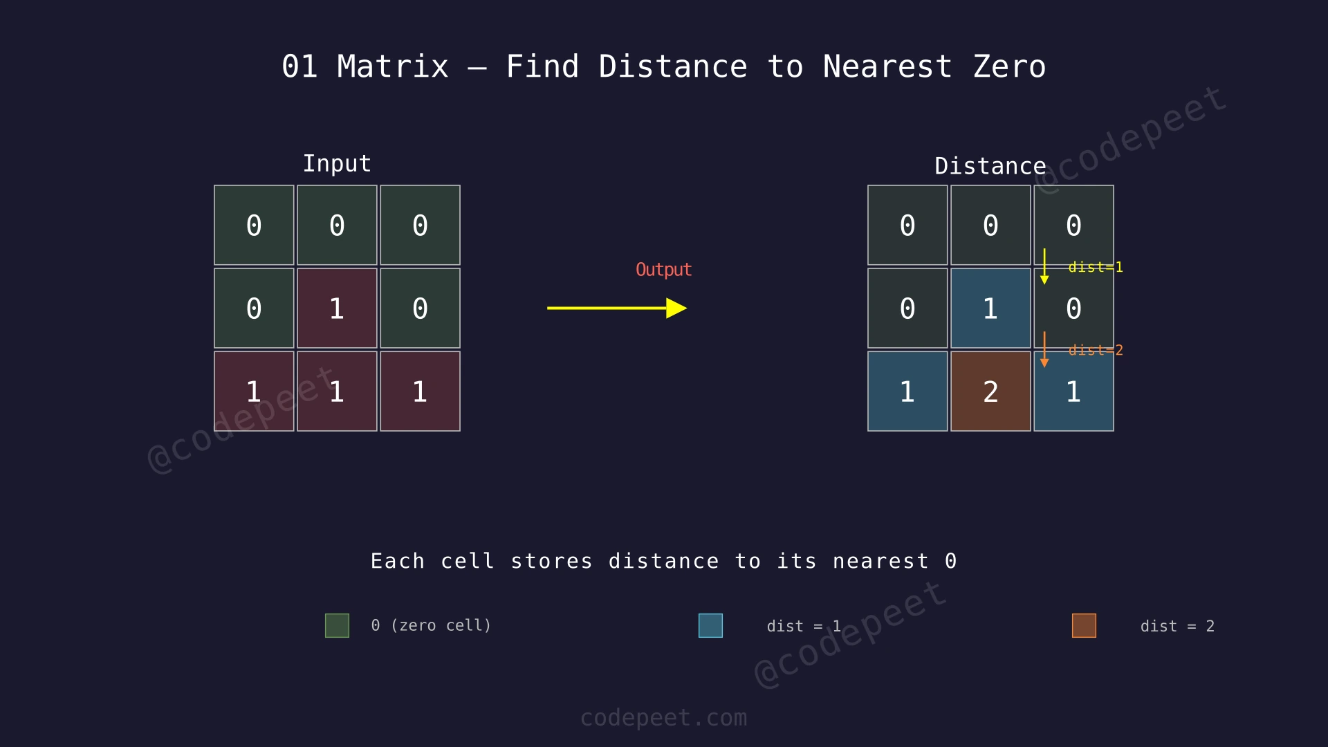
You are given an m × n binary matrix mat where each cell contains either a 0 or a 1. Your task is to find, for every cell in the matrix, the distance to the nearest cell containing 0.
The distance between two adjacent cells (cells sharing a common edge — up, down, left, or right) is exactly 1. Diagonal movement is not allowed. So the distance between any two cells is the Manhattan distance: the sum of the absolute differences of their row and column indices.
In other words, for every cell (i, j) in the matrix:
- If
mat[i][j] == 0, the answer for that cell is0(distance to itself). - If
mat[i][j] == 1, the answer is the minimum number of horizontal/vertical steps required to reach any cell containing0.
Examples
Example 1
Input: mat = [[0,0,0],[0,1,0],[0,0,0]]
Output: [[0,0,0],[0,1,0],[0,0,0]]
Explanation: The only cell containing 1 is at position (1,1). Its four immediate neighbors — (0,1), (1,0), (1,2), and (2,1) — all contain 0. The shortest distance from (1,1) to any of these is 1. Every cell containing 0 has distance 0 to itself.
Example 2
Input: mat = [[0,0,0],[0,1,0],[1,1,1]]
Output: [[0,0,0],[0,1,0],[1,2,1]]
Explanation: Cells in the top row are all 0, so their distances are all 0. Cell (1,0) and (1,2) are 0, so their distances are 0. Cell (1,1) is 1 and its nearest 0 is one step away (e.g., at (0,1) or (1,0)), so its distance is 1. Cell (2,0) is 1 and the nearest 0 is at (1,0), one step above — distance 1. Cell (2,1) is 1 and the nearest 0 is two steps away (e.g., through (1,1) to (0,1)), so distance is 2. Cell (2,2) is 1 and the nearest 0 is at (1,2), one step above — distance 1.
Constraints
- m == mat.length
- n == mat[i].length
- 1 ≤ m, n ≤ 10^4
- 1 ≤ m × n ≤ 10^4
- mat[i][j] is either 0 or 1
- There is at least one 0 in mat
Editorial
Brute Force
Intuition
The most straightforward way to think about this problem is: for each cell that contains a 1, look at every single cell in the entire matrix, find all the 0-cells, compute the Manhattan distance to each of them, and keep the smallest distance.
Imagine you are standing on a 1-cell in a giant grid-shaped city. You need to find the nearest hospital (a 0-cell). The brute force way is to check every single building in the city, measure how far it is, and note down the closest hospital. Then you move to the next 1-cell and repeat the entire city-wide search.
For cells that already contain 0, the answer is trivially 0 — they are hospitals themselves.
Step-by-Step Explanation
Let's trace through with mat = [[0,0,0],[0,1,0],[1,1,1]]:
We initialize a result matrix of the same size, filled with a large value (infinity).
Step 1: Process cell (0,0). mat[0][0] = 0, so result[0][0] = 0. No scanning needed.
- result = [[0, ∞, ∞], [∞, ∞, ∞], [∞, ∞, ∞]]
Step 2: Process cells (0,1), (0,2), (1,0), (1,2). All are 0-cells, so their result is 0.
- result = [[0, 0, 0], [0, ∞, 0], [∞, ∞, ∞]]
Step 3: Process cell (1,1). mat[1][1] = 1. Scan all cells for 0s:
- (0,0) is 0: distance = |1-0| + |1-0| = 2
- (0,1) is 0: distance = |1-0| + |1-1| = 1
- (0,2) is 0: distance = |1-0| + |1-2| = 2
- (1,0) is 0: distance = |1-1| + |1-0| = 1
- (1,2) is 0: distance = |1-1| + |1-2| = 1
- Minimum = 1. Set result[1][1] = 1.
- result = [[0, 0, 0], [0, 1, 0], [∞, ∞, ∞]]
Step 4: Process cell (2,0). mat[2][0] = 1. Scan all cells for 0s:
- (0,0) is 0: distance = |2-0| + |0-0| = 2
- (0,1) is 0: distance = |2-0| + |0-1| = 3
- (0,2) is 0: distance = |2-0| + |0-2| = 4
- (1,0) is 0: distance = |2-1| + |0-0| = 1
- (1,2) is 0: distance = |2-1| + |0-2| = 3
- Minimum = 1. Set result[2][0] = 1.
- result = [[0, 0, 0], [0, 1, 0], [1, ∞, ∞]]
Step 5: Process cell (2,1). mat[2][1] = 1. Scan all cells for 0s:
- (0,0) is 0: distance = |2-0| + |1-0| = 3
- (0,1) is 0: distance = |2-0| + |1-1| = 2
- (0,2) is 0: distance = |2-0| + |1-2| = 3
- (1,0) is 0: distance = |2-1| + |1-0| = 2
- (1,2) is 0: distance = |2-1| + |1-2| = 2
- Minimum = 2. Set result[2][1] = 2.
- result = [[0, 0, 0], [0, 1, 0], [1, 2, ∞]]
Step 6: Process cell (2,2). mat[2][2] = 1. Scan all cells for 0s:
- (0,0) is 0: distance = |2-0| + |2-0| = 4
- (0,1) is 0: distance = |2-0| + |2-1| = 3
- (0,2) is 0: distance = |2-0| + |2-2| = 2
- (1,0) is 0: distance = |2-1| + |2-0| = 3
- (1,2) is 0: distance = |2-1| + |2-2| = 1
- Minimum = 1. Set result[2][2] = 1.
- result = [[0, 0, 0], [0, 1, 0], [1, 2, 1]]
Result: [[0, 0, 0], [0, 1, 0], [1, 2, 1]]
Algorithm
- Create a result matrix of size m × n, initialized with a very large value (infinity).
- For each cell (i, j) in the matrix:
- If mat[i][j] == 0, set result[i][j] = 0.
- If mat[i][j] == 1, iterate over every cell (r, c) in the matrix:
- If mat[r][c] == 0, compute distance = |i - r| + |j - c|.
- Update result[i][j] = min(result[i][j], distance).
- Return the result matrix.
Code
class Solution {
public:
    vector<vector<int>> updateMatrix(vector<vector<int>>& mat) {
        int m = mat.size(), n = mat[0].size();
        vector<vector<int>> result(m, vector<int>(n, INT_MAX));

        for (int i = 0; i < m; i++) {
            for (int j = 0; j < n; j++) {
                if (mat[i][j] == 0) {
                    result[i][j] = 0;
                } else {
                    for (int r = 0; r < m; r++) {
                        for (int c = 0; c < n; c++) {
                            if (mat[r][c] == 0) {
                                result[i][j] = min(result[i][j],
                                    abs(i - r) + abs(j - c));
                            }
                        }
                    }
                }
            }
        }
        return result;
    }
};
class Solution:
def updateMatrix(self, mat: list[list[int]]) -> list[list[int]]:
m, n = len(mat), len(mat[0])
result = [[float('inf')] * n for _ in range(m)]
for i in range(m):
for j in range(n):
if mat[i][j] == 0:
result[i][j] = 0
else:
for r in range(m):
for c in range(n):
if mat[r][c] == 0:
result[i][j] = min(
result[i][j],
abs(i - r) + abs(j - c)
)
return resultclass Solution {
public int[][] updateMatrix(int[][] mat) {
int m = mat.length, n = mat[0].length;
int[][] result = new int[m][n];
for (int[] row : result) {
Arrays.fill(row, Integer.MAX_VALUE);
}
for (int i = 0; i < m; i++) {
for (int j = 0; j < n; j++) {
if (mat[i][j] == 0) {
result[i][j] = 0;
} else {
for (int r = 0; r < m; r++) {
for (int c = 0; c < n; c++) {
if (mat[r][c] == 0) {
result[i][j] = Math.min(
result[i][j],
Math.abs(i - r) + Math.abs(j - c)
);
}
}
}
}
}
}
return result;
}
}Complexity Analysis
Time Complexity: O((m × n)²)
For each of the m × n cells, if it contains a 1, we scan the entire m × n matrix to find the nearest 0. In the worst case (all cells are 1 except one), every cell performs a full matrix scan. This gives us O(m × n) cells × O(m × n) scan per cell = O((m × n)²).
Space Complexity: O(m × n)
We use a result matrix of the same dimensions as the input. No other data structures grow with input size.
Why This Approach Is Not Efficient
The brute force approach has a time complexity of O((m × n)²). With the constraint that m × n can be up to 10,000, this translates to up to 10^8 operations — right at the edge of typical time limits and very likely to cause a Time Limit Exceeded verdict.
The fundamental inefficiency is redundant scanning. When we compute the distance for cell (2,1), we scan every cell in the matrix. When we move to cell (2,2), we scan the entire matrix again. But these two cells share many of the same nearby 0 sources. We are throwing away all the work we did for one cell when we start processing the next.
The key insight is to flip the perspective: instead of starting from each 1 and searching for the nearest 0, we can start from all 0-cells simultaneously and expand outward. This way, each cell is visited only once, and the first time a 1-cell is reached by this expansion, it receives its minimum distance. This is the essence of multi-source BFS.
Better Approach - Multi-Source BFS
Intuition
Instead of searching for the nearest 0 from each 1-cell, we reverse the problem. We start from all 0-cells at once and expand outward like ripples in a pond.
Imagine dropping a stone into a pond at every location where there is a 0. All the stones hit the water at the same time, and ripples spread outward simultaneously. When two ripples from different stones collide, they stop — because the cell has already been reached by a closer stone. The number of ripple waves it takes to reach any particular cell is exactly the shortest distance to the nearest 0.
This is called multi-source BFS (Breadth-First Search). We initialize a queue with all 0-cells (distance 0), then process them level by level. At each level, we discover new cells one step farther away. Because BFS explores cells in order of increasing distance, the first time we reach any 1-cell, we have found its shortest distance to a 0.
Step-by-Step Explanation
Let's trace through with mat = [[0,0,0],[0,1,0],[1,1,1]]:
Step 1: Initialization. Create a distance matrix. Set distance = 0 for all 0-cells, and distance = ∞ for all 1-cells. Enqueue all 0-cells.
- Distance grid: [[0, 0, 0], [0, ∞, 0], [∞, ∞, ∞]]
- Queue: [(0,0), (0,1), (0,2), (1,0), (1,2)]
Step 2: Dequeue (0,0). Distance is 0. Check neighbors:
- (0,1) → already distance 0. Skip.
- (1,0) → already distance 0. Skip.
- No unvisited neighbors to update.
Step 3: Dequeue (0,1). Distance is 0. Check neighbors:
- (0,0) → distance 0, skip.
- (0,2) → distance 0, skip.
- (1,1) → distance ∞! Update to 0 + 1 = 1. Enqueue (1,1).
- Distance grid: [[0, 0, 0], [0, 1, 0], [∞, ∞, ∞]]
Step 4: Dequeue (0,2). Distance is 0. Check neighbors:
- (0,1) → distance 0, skip.
- (1,2) → distance 0, skip.
- No unvisited neighbors.
Step 5: Dequeue (1,0). Distance is 0. Check neighbors:
- (0,0) → distance 0, skip.
- (1,1) → distance 1, already updated. Skip.
- (2,0) → distance ∞! Update to 0 + 1 = 1. Enqueue (2,0).
- Distance grid: [[0, 0, 0], [0, 1, 0], [1, ∞, ∞]]
Step 6: Dequeue (1,2). Distance is 0. Check neighbors:
- (0,2) → distance 0, skip.
- (1,1) → distance 1, skip.
- (2,2) → distance ∞! Update to 0 + 1 = 1. Enqueue (2,2).
- Distance grid: [[0, 0, 0], [0, 1, 0], [1, ∞, 1]]
Step 7: Dequeue (1,1). Distance is 1. Check neighbors:
- (0,1) → distance 0, skip.
- (1,0) → distance 0, skip.
- (1,2) → distance 0, skip.
- (2,1) → distance ∞! Update to 1 + 1 = 2. Enqueue (2,1).
- Distance grid: [[0, 0, 0], [0, 1, 0], [1, 2, 1]]
Step 8: Process remaining cells. (2,0), (2,2), and (2,1) are dequeued. Their neighbors all have distances already assigned. No further updates.
Step 9: Queue empty. BFS complete.
- Final result: [[0, 0, 0], [0, 1, 0], [1, 2, 1]]
Multi-Source BFS — Ripple Expansion from All Zeros — Watch how BFS starts from all 0-cells simultaneously and expands outward layer by layer, assigning each 1-cell its minimum distance to the nearest 0.
Algorithm
- Create a distance matrix
distof size m × n, initialized to ∞ (or -1 as an unvisited marker). - Create an empty queue.
- Iterate over every cell (i, j):
- If mat[i][j] == 0, set dist[i][j] = 0 and enqueue (i, j).
- While the queue is not empty:
- Dequeue a cell (r, c).
- For each of the 4 neighbors (nr, nc) — up, down, left, right:
- If (nr, nc) is within bounds and dist[nr][nc] > dist[r][c] + 1:
- Update dist[nr][nc] = dist[r][c] + 1.
- Enqueue (nr, nc).
- If (nr, nc) is within bounds and dist[nr][nc] > dist[r][c] + 1:
- Return dist.
Code
class Solution {
public:
    vector<vector<int>> updateMatrix(vector<vector<int>>& mat) {
        int m = mat.size(), n = mat[0].size();
        vector<vector<int>> dist(m, vector<int>(n, INT_MAX));
        queue<pair<int, int>> q;

        for (int i = 0; i < m; i++) {
            for (int j = 0; j < n; j++) {
                if (mat[i][j] == 0) {
                    dist[i][j] = 0;
                    q.push({i, j});
                }
            }
        }

        int dirs[4][2] = {{-1,0},{1,0},{0,-1},{0,1}};

        while (!q.empty()) {
            auto [r, c] = q.front();
            q.pop();
            for (auto& d : dirs) {
                int nr = r + d[0], nc = c + d[1];
                if (nr >= 0 && nr < m && nc >= 0 && nc < n
                    && dist[nr][nc] > dist[r][c] + 1) {
                    dist[nr][nc] = dist[r][c] + 1;
                    q.push({nr, nc});
                }
            }
        }
        return dist;
    }
};
from collections import deque
class Solution:
def updateMatrix(self, mat: list[list[int]]) -> list[list[int]]:
m, n = len(mat), len(mat[0])
dist = [[float('inf')] * n for _ in range(m)]
q = deque()
for i in range(m):
for j in range(n):
if mat[i][j] == 0:
dist[i][j] = 0
q.append((i, j))
directions = [(-1, 0), (1, 0), (0, -1), (0, 1)]
while q:
r, c = q.popleft()
for dr, dc in directions:
nr, nc = r + dr, c + dc
if 0 <= nr < m and 0 <= nc < n \
and dist[nr][nc] > dist[r][c] + 1:
dist[nr][nc] = dist[r][c] + 1
q.append((nr, nc))
return distclass Solution {
public int[][] updateMatrix(int[][] mat) {
int m = mat.length, n = mat[0].length;
int[][] dist = new int[m][n];
Queue<int[]> queue = new LinkedList<>();
for (int[] row : dist) {
Arrays.fill(row, Integer.MAX_VALUE);
}
for (int i = 0; i < m; i++) {
for (int j = 0; j < n; j++) {
if (mat[i][j] == 0) {
dist[i][j] = 0;
queue.offer(new int[]{i, j});
}
}
}
int[][] dirs = {{-1,0},{1,0},{0,-1},{0,1}};
while (!queue.isEmpty()) {
int[] cell = queue.poll();
int r = cell[0], c = cell[1];
for (int[] d : dirs) {
int nr = r + d[0], nc = c + d[1];
if (nr >= 0 && nr < m && nc >= 0 && nc < n
&& dist[nr][nc] > dist[r][c] + 1) {
dist[nr][nc] = dist[r][c] + 1;
queue.offer(new int[]{nr, nc});
}
}
}
return dist;
}
}Complexity Analysis
Time Complexity: O(m × n)
Every cell is enqueued and dequeued at most once. When a cell is processed, we check its 4 neighbors — a constant amount of work. So the total work is proportional to the number of cells: O(m × n).
Space Complexity: O(m × n)
The distance matrix uses O(m × n) space. The BFS queue can hold up to O(m × n) cells in the worst case (when all cells are 0, they are all enqueued initially). Thus, total space is O(m × n).
Why This Approach Is Not Efficient
The multi-source BFS approach is already excellent in terms of time complexity — O(m × n) is optimal since we must examine every cell at least once. However, it requires O(m × n) extra space for the BFS queue.
In the worst case, the queue can contain a significant fraction of all cells (e.g., if most cells are 0, they are all enqueued during initialization). While this space usage is acceptable for most practical inputs, we can ask: is it possible to achieve the same O(m × n) time without maintaining an explicit queue?
The answer is yes. A dynamic programming approach can compute the same result using only the output matrix itself — no queue, no visited array, no extra data structure beyond what we return. This reduces the auxiliary space to O(1), which is as space-efficient as possible.
Optimal Approach - Dynamic Programming (Two-Pass)
Intuition
The DP approach relies on a crucial observation: the distance to the nearest 0 for any cell can be decomposed into the distances along specific directions.
Think of it this way: if you are at cell (i, j) and the nearest 0 is somewhere above-left of you, then the shortest path to it goes through either your top neighbor or your left neighbor. Similarly, if the nearest 0 is below-right, the shortest path goes through your bottom or right neighbor.
No single left-to-right scan can capture distances from 0-cells in all directions. But two passes can:
-
First pass (top-left → bottom-right): For each cell, compute the minimum distance considering only
0-cells that are above or to the left. We look at the top neighbor and the left neighbor. -
Second pass (bottom-right → top-left): For each cell, refine the distance considering
0-cells that are below or to the right. We look at the bottom neighbor and the right neighbor.
After both passes, every cell has the correct minimum distance because every possible direction to a 0-cell has been considered. The first pass handles the "northwest" contribution, and the second pass handles the "southeast" contribution. Together, they cover all four directions.
Step-by-Step Explanation
Let's trace through with mat = [[0,0,0],[0,1,0],[1,1,1]]:
Step 1: Initialize. Set dist[i][j] = 0 if mat[i][j] == 0, else ∞.
- dist = [[0, 0, 0], [0, ∞, 0], [∞, ∞, ∞]]
--- First Pass: Top-left → Bottom-right ---
Step 2: Process (0,0) through (1,0). These are all 0-cells, so they stay at 0. Skip to the first interesting cell.
- dist = [[0, 0, 0], [0, ∞, 0], [∞, ∞, ∞]]
Step 3: Process (1,1). Current = ∞. Check:
- Top neighbor (0,1) = 0 → 0 + 1 = 1
- Left neighbor (1,0) = 0 → 0 + 1 = 1
- min(∞, 1, 1) = 1. Update dist[1][1] = 1.
- dist = [[0, 0, 0], [0, 1, 0], [∞, ∞, ∞]]
Step 4: Process (2,0). Current = ∞. Check:
- Top neighbor (1,0) = 0 → 0 + 1 = 1
- No left neighbor (out of bounds).
- min(∞, 1) = 1. Update dist[2][0] = 1.
- dist = [[0, 0, 0], [0, 1, 0], [1, ∞, ∞]]
Step 5: Process (2,1). Current = ∞. Check:
- Top neighbor (1,1) = 1 → 1 + 1 = 2
- Left neighbor (2,0) = 1 → 1 + 1 = 2
- min(∞, 2, 2) = 2. Update dist[2][1] = 2.
- dist = [[0, 0, 0], [0, 1, 0], [1, 2, ∞]]
Step 6: Process (2,2). Current = ∞. Check:
- Top neighbor (1,2) = 0 → 0 + 1 = 1
- Left neighbor (2,1) = 2 → 2 + 1 = 3
- min(∞, 1, 3) = 1. Update dist[2][2] = 1.
- dist = [[0, 0, 0], [0, 1, 0], [1, 2, 1]]
--- Second Pass: Bottom-right → Top-left ---
Step 7: Process (2,2). Current = 1. No bottom or right neighbor. No change.
Step 8: Process (2,1). Current = 2. Check:
- Right neighbor (2,2) = 1 → 1 + 1 = 2.
- min(2, 2) = 2. No change. The first pass already found the optimal distance.
Step 9: Process (1,1). Current = 1. Check:
- Bottom neighbor (2,1) = 2 → 2 + 1 = 3.
- Right neighbor (1,2) = 0 → 0 + 1 = 1.
- min(1, 3, 1) = 1. No change — value is already correct.
Step 10: Complete. All cells confirmed.
- Final result: [[0, 0, 0], [0, 1, 0], [1, 2, 1]]
DP Two-Pass — Forward and Backward Sweeps — Watch the two-pass DP approach: the first pass propagates distances from top-left 0-cells, and the second pass refines them from bottom-right 0-cells.
Algorithm
- Create a distance matrix
distof size m × n. - Initialize: for each cell, if mat[i][j] == 0, set dist[i][j] = 0; otherwise set dist[i][j] = a large value (e.g., m + n, since no distance can exceed m + n - 2).
- First pass (top-left → bottom-right): For each cell (i, j) in row-major order:
- If i > 0: dist[i][j] = min(dist[i][j], dist[i-1][j] + 1) (check top)
- If j > 0: dist[i][j] = min(dist[i][j], dist[i][j-1] + 1) (check left)
- Second pass (bottom-right → top-left): For each cell (i, j) in reverse row-major order:
- If i < m-1: dist[i][j] = min(dist[i][j], dist[i+1][j] + 1) (check bottom)
- If j < n-1: dist[i][j] = min(dist[i][j], dist[i][j+1] + 1) (check right)
- Return dist.
Code
class Solution {
public:
    vector<vector<int>> updateMatrix(vector<vector<int>>& mat) {
        int m = mat.size(), n = mat[0].size();
        int INF = m + n;
        vector<vector<int>> dist(m, vector<int>(n, INF));

        // First pass: top-left to bottom-right
        for (int i = 0; i < m; i++) {
            for (int j = 0; j < n; j++) {
                if (mat[i][j] == 0) {
                    dist[i][j] = 0;
                } else {
                    if (i > 0)
                        dist[i][j] = min(dist[i][j], dist[i-1][j] + 1);
                    if (j > 0)
                        dist[i][j] = min(dist[i][j], dist[i][j-1] + 1);
                }
            }
        }

        // Second pass: bottom-right to top-left
        for (int i = m - 1; i >= 0; i--) {
            for (int j = n - 1; j >= 0; j--) {
                if (i < m - 1)
                    dist[i][j] = min(dist[i][j], dist[i+1][j] + 1);
                if (j < n - 1)
                    dist[i][j] = min(dist[i][j], dist[i][j+1] + 1);
            }
        }

        return dist;
    }
};
class Solution:
def updateMatrix(self, mat: list[list[int]]) -> list[list[int]]:
m, n = len(mat), len(mat[0])
INF = m + n
dist = [[INF] * n for _ in range(m)]
# First pass: top-left to bottom-right
for i in range(m):
for j in range(n):
if mat[i][j] == 0:
dist[i][j] = 0
else:
if i > 0:
dist[i][j] = min(dist[i][j], dist[i - 1][j] + 1)
if j > 0:
dist[i][j] = min(dist[i][j], dist[i][j - 1] + 1)
# Second pass: bottom-right to top-left
for i in range(m - 1, -1, -1):
for j in range(n - 1, -1, -1):
if i < m - 1:
dist[i][j] = min(dist[i][j], dist[i + 1][j] + 1)
if j < n - 1:
dist[i][j] = min(dist[i][j], dist[i][j + 1] + 1)
return distclass Solution {
public int[][] updateMatrix(int[][] mat) {
int m = mat.length, n = mat[0].length;
int INF = m + n;
int[][] dist = new int[m][n];
for (int[] row : dist) {
Arrays.fill(row, INF);
}
// First pass: top-left to bottom-right
for (int i = 0; i < m; i++) {
for (int j = 0; j < n; j++) {
if (mat[i][j] == 0) {
dist[i][j] = 0;
} else {
if (i > 0)
dist[i][j] = Math.min(dist[i][j], dist[i - 1][j] + 1);
if (j > 0)
dist[i][j] = Math.min(dist[i][j], dist[i][j - 1] + 1);
}
}
}
// Second pass: bottom-right to top-left
for (int i = m - 1; i >= 0; i--) {
for (int j = n - 1; j >= 0; j--) {
if (i < m - 1)
dist[i][j] = Math.min(dist[i][j], dist[i + 1][j] + 1);
if (j < n - 1)
dist[i][j] = Math.min(dist[i][j], dist[i][j + 1] + 1);
}
}
return dist;
}
}Complexity Analysis
Time Complexity: O(m × n)
We make exactly two passes over the matrix. Each pass visits every cell once and performs a constant amount of work (two comparisons and a min operation). Total: 2 × O(m × n) = O(m × n).
Space Complexity: O(1) auxiliary space
The only extra space we use is the output distance matrix, which the problem requires us to return. Beyond that, we use a fixed number of integer variables. No queue, no visited array, no additional data structures. If we count the output space, it is O(m × n), but the auxiliary (extra) space is O(1).
This makes the DP approach the most space-efficient solution while maintaining the same optimal O(m × n) time as multi-source BFS.