Bellman-Ford Algorithm
Description
You are given a weighted directed graph with V vertices (numbered 0 to V-1) and E directed edges. Each edge is described by three values: a source vertex, a destination vertex, and a weight (which can be negative).
Given a starting vertex src, compute the shortest distance from src to every other vertex in the graph.
Special conditions:
- If a vertex is not reachable from the source, report its distance as 10^8 (representing infinity).
- If the graph contains a negative weight cycle reachable from the source (a cycle where the sum of edge weights is negative), return [-1]. A negative cycle makes shortest paths undefined because you could loop through the cycle infinitely to keep reducing the total path weight.
This problem specifically requires handling negative edge weights, which many simpler shortest-path algorithms (like Dijkstra's) cannot handle correctly.
Examples
Example 1
Input: V = 5, edges = [[0, 1, 5], [1, 2, 1], [1, 3, 2], [2, 4, 1], [4, 3, -1]], src = 0
Output: [0, 5, 6, 6, 7]
Explanation:
- Distance to vertex 0: 0 (source itself)
- Distance to vertex 1: 5 (path: 0 → 1, weight = 5)
- Distance to vertex 2: 6 (path: 0 → 1 → 2, weight = 5 + 1 = 6)
- Distance to vertex 3: 6 (path: 0 → 1 → 2 → 4 → 3, weight = 5 + 1 + 1 + (-1) = 6). Note that the direct path 0 → 1 → 3 has weight 7, but taking the detour through vertex 4 with the negative edge gives weight 6, which is shorter.
- Distance to vertex 4: 7 (path: 0 → 1 → 2 → 4, weight = 5 + 1 + 1 = 7)
Example 2
Input: V = 4, edges = [[0, 1, 4], [1, 2, -6], [2, 3, 5], [3, 1, -2]], src = 0
Output: [-1]
Explanation:
The graph contains a negative weight cycle: 1 → 2 → 3 → 1. The total weight of this cycle is (-6) + 5 + (-2) = -3. Every time you traverse this cycle, the total path weight decreases by 3. This means you could keep going around the cycle forever, making the "shortest" distance arbitrarily small (negative infinity). Therefore, finite shortest paths do not exist, and we return [-1].
Example 3
Input: V = 3, edges = [[0, 1, 2], [1, 2, 3]], src = 0
Output: [0, 2, 5]
Explanation:
- Distance to vertex 0: 0 (source)
- Distance to vertex 1: 2 (path: 0 → 1, weight = 2)
- Distance to vertex 2: 5 (path: 0 → 1 → 2, weight = 2 + 3 = 5)
A simple case with only positive weights. No negative edges, no cycles.
Constraints
- 1 ≤ V ≤ 500
- 1 ≤ E ≤ V × (V - 1)
- -1000 ≤ edge weight ≤ 1000
- 0 ≤ src < V
- No self-loops
- The graph is directed
- There may be negative weight edges
- Unreachable vertices should have distance 10^8
Editorial
Brute Force
Intuition
The most natural way to think about finding the shortest path is: just try every possible route from the source to each destination and pick the shortest one.
Imagine you are in a city and want to find the cheapest flight route from your city to every other city. The brute force approach is like checking every single combination of connecting flights, calculating the total cost for each route, and then choosing the cheapest one for each destination.
In graph terms, for each destination vertex, we perform a Depth-First Search (DFS) starting from the source. We explore every possible simple path (a path that never revisits a vertex) and keep track of the minimum total weight among all paths that reach the destination.
We use backtracking to ensure we explore all possibilities: after visiting a vertex along one path, we "unvisit" it so it can be used in other paths.
Important limitation: This approach only considers simple paths (no repeated vertices), so it inherently cannot detect negative weight cycles. The DFS avoids revisiting vertices, which means it never traverses a cycle. For graphs with negative cycles, this approach would return finite distances that are actually incorrect — the true shortest distances should be negative infinity.
Step-by-Step Explanation
Let's trace through Example 1: V = 5, edges = [[0,1,5], [1,2,1], [1,3,2], [2,4,1], [4,3,-1]], src = 0.
First, build the adjacency list:
- Vertex 0 → [(1, 5)]
- Vertex 1 → [(2, 1), (3, 2)]
- Vertex 2 → [(4, 1)]
- Vertex 3 → [] (no outgoing edges)
- Vertex 4 → [(3, -1)]
Step 1: Initialize dist = [0, 10^8, 10^8, 10^8, 10^8]. Source vertex 0 has distance 0.
Step 2: Find shortest path from 0 to vertex 1.
- DFS from 0, visited = {0}
- Go to neighbor 1 (edge weight 5): path cost = 0 + 5 = 5
- Reached vertex 1! Record cost = 5
- No more paths to explore.
- Shortest distance to vertex 1 = 5
- dist = [0, 5, 10^8, 10^8, 10^8]
Step 3: Find shortest path from 0 to vertex 2.
- DFS from 0, visited = {0}
- Go to 1 (cost 5), visited = {0, 1}
- Go to 2 (cost 5+1=6), visited = {0, 1, 2}
- Reached vertex 2! Record cost = 6
- Go to 3 (cost 5+2=7), visited = {0, 1, 3}
- Vertex 3 has no outgoing edges — dead end
- Backtrack
- Go to 2 (cost 5+1=6), visited = {0, 1, 2}
- All paths explored. Shortest = 6
- dist = [0, 5, 6, 10^8, 10^8]
Step 4: Find shortest path from 0 to vertex 3.
- DFS from 0, visited = {0}
- Go to 1 (cost 5), visited = {0, 1}
- Go to 2 (cost 6), visited = {0, 1, 2}
- Go to 4 (cost 7), visited = {0, 1, 2, 4}
- Go to 3 (cost 7 + (-1) = 6), visited = {0, 1, 2, 4, 3}
- Reached vertex 3! Record cost = 6
- Go to 3 (cost 7 + (-1) = 6), visited = {0, 1, 2, 4, 3}
- Go to 4 (cost 7), visited = {0, 1, 2, 4}
- Go to 3 (cost 5+2=7), visited = {0, 1, 3}
- Reached vertex 3! Record cost = 7
- Go to 2 (cost 6), visited = {0, 1, 2}
- All paths explored. Shortest = min(6, 7) = 6
- dist = [0, 5, 6, 6, 10^8]
Step 5: Find shortest path from 0 to vertex 4.
- DFS from 0, visited = {0}
- Go to 1 (cost 5), visited = {0, 1}
- Go to 2 (cost 6), visited = {0, 1, 2}
- Go to 4 (cost 7), visited = {0, 1, 2, 4}
- Reached vertex 4! Record cost = 7
- (Neighbor 3 exists but is not vertex 4)
- Go to 4 (cost 7), visited = {0, 1, 2, 4}
- Go to 3 (cost 7), visited = {0, 1, 3}
- Vertex 3 has no outgoing edges — cannot reach 4 from here
- Go to 2 (cost 6), visited = {0, 1, 2}
- All paths explored. Shortest = 7
- dist = [0, 5, 6, 6, 7]
Step 6: Final result = [0, 5, 6, 6, 7]. We explored all simple paths for each vertex.
Algorithm
- Build an adjacency list from the edge list.
- Initialize a distance array of size V, with all values set to 10^8 (infinity), except dist[src] = 0.
- For each destination vertex d (where d ≠ src):
a. Perform DFS with backtracking from the source vertex.
b. Track a visited set to avoid revisiting vertices (ensuring only simple paths).
c. At each recursive call, add the edge weight to the running cost.
d. When the destination is reached, update the minimum distance if the current path cost is smaller.
e. After exploring a neighbor, remove it from the visited set (backtrack). - Return the distance array.
Note: This approach cannot detect negative weight cycles because it only considers simple paths.
Code
#include <vector>
#include <climits>
#include <algorithm>
using namespace std;

class Solution {
    void dfs(int node, int dest, int cost, int& best,
             vector<vector<pair<int,int>>>& adj, vector<bool>& vis) {
        if (node == dest) {
            best = min(best, cost);
            return;
        }
        vis[node] = true;
        for (auto& [next, w] : adj[node]) {
            if (!vis[next]) {
                dfs(next, dest, cost + w, best, adj, vis);
            }
        }
        vis[node] = false;
    }

public:
    vector<int> shortestPath(int V, vector<vector<int>>& edges, int src) {
        vector<vector<pair<int,int>>> adj(V);
        for (auto& e : edges) {
            adj[e[0]].push_back({e[1], e[2]});
        }

        vector<int> dist(V, 1e8);
        dist[src] = 0;

        for (int d = 0; d < V; d++) {
            if (d == src) continue;
            int best = 1e8;
            vector<bool> vis(V, false);
            dfs(src, d, 0, best, adj, vis);
            dist[d] = best;
        }

        return dist;
    }
};
class Solution:
def shortestPath(self, V, edges, src):
adj = [[] for _ in range(V)]
for u, v, w in edges:
adj[u].append((v, w))
dist = [10**8] * V
dist[src] = 0
def dfs(node, dest, cost, visited):
if node == dest:
return cost
visited.add(node)
best = 10**8
for next_node, weight in adj[node]:
if next_node not in visited:
best = min(best, dfs(next_node, dest, cost + weight, visited))
visited.remove(node)
return best
for d in range(V):
if d == src:
continue
dist[d] = dfs(src, d, 0, set())
return distimport java.util.*;
class Solution {
int best;
void dfs(int node, int dest, int cost,
List<List<int[]>> adj, boolean[] vis) {
if (node == dest) {
best = Math.min(best, cost);
return;
}
vis[node] = true;
for (int[] next : adj.get(node)) {
if (!vis[next[0]]) {
dfs(next[0], dest, cost + next[1], adj, vis);
}
}
vis[node] = false;
}
public int[] shortestPath(int V, int[][] edges, int src) {
List<List<int[]>> adj = new ArrayList<>();
for (int i = 0; i < V; i++) adj.add(new ArrayList<>());
for (int[] e : edges) {
adj.get(e[0]).add(new int[]{e[1], e[2]});
}
int[] dist = new int[V];
Arrays.fill(dist, (int)1e8);
dist[src] = 0;
for (int d = 0; d < V; d++) {
if (d == src) continue;
best = (int)1e8;
boolean[] vis = new boolean[V];
dfs(src, d, 0, adj, vis);
dist[d] = best;
}
return dist;
}
}Complexity Analysis
Time Complexity: O(V × V!)
For each of the V destination vertices, we perform a DFS that explores all simple paths. In the worst case (a complete graph where every vertex connects to every other vertex), the number of simple paths from source to any destination can be factorial — up to (V-1)! paths. Each path can have up to V-1 edges. So the total work is approximately O(V × V!), which is exponential.
For V = 500, this is astronomically large and completely infeasible.
Space Complexity: O(V)
The recursion stack can go at most V levels deep (one level per vertex in the longest simple path). The visited set also uses O(V) space. The adjacency list uses O(V + E) space for storage.
Why This Approach Is Not Efficient
The brute force approach has two critical problems:
1. Exponential Time Complexity
Exploring all simple paths is an exponential operation. For a graph with V = 500 vertices and a dense edge set, the number of possible simple paths grows factorially. Even for V = 20, there could be trillions of paths to examine. The constraint allows V up to 500, making this approach entirely impractical.
2. Cannot Detect Negative Weight Cycles
Because DFS with backtracking only considers simple paths (paths that visit each vertex at most once), it never traverses a cycle. This means it cannot detect negative weight cycles — a core requirement of the problem. It would incorrectly return finite distances even when the true shortest distances should be undefined (negative infinity).
The Key Insight for Improvement:
Instead of trying every possible path, we can use a powerful observation about shortest paths: a shortest simple path in a graph with V vertices has at most V-1 edges. If we could systematically "relax" (improve) distances by considering edges one at a time, repeating this process V-1 times would guarantee that the shortest path information has propagated through the entire graph. This is the principle behind the Bellman-Ford algorithm, which reduces the time from exponential to polynomial O(V × E).
Optimal Approach - Bellman-Ford (Edge Relaxation)
Intuition
Instead of exploring every possible path (which is exponential), the Bellman-Ford algorithm uses a brilliant shortcut based on one key insight:
Any shortest path in a graph with V vertices uses at most V-1 edges.
Why? Because a shortest path never revisits a vertex (if it did, it would contain a cycle, and unless that cycle has negative total weight, removing the cycle would give an equal or shorter path). Since there are only V vertices, any simple path has at most V-1 edges.
This insight leads to a elegant strategy called edge relaxation:
Relaxation means: for an edge (u → v) with weight w, if the current known distance to v is longer than the distance to u plus w, then we have found a better route to v through u. We update dist[v] = dist[u] + w.
The algorithm works in rounds. In each round, it scans through ALL edges and tries to relax each one. After one round, we are guaranteed to know the correct shortest distances for all vertices reachable within 1 edge from the source. After two rounds, we know distances for all vertices within 2 edges. After V-1 rounds, we know ALL shortest distances.
Think of it like ripples spreading outward from a stone dropped in water. Each iteration of relaxation lets the shortest-path information "travel" one more edge further from the source.
Negative cycle detection comes as a bonus: if, after V-1 rounds, a V-th round still produces an improvement, it means some distance is still decreasing — which is only possible if a negative cycle exists.
Step-by-Step Explanation
Let's trace Example 1: V = 5, edges = [[0,1,5], [1,2,1], [1,3,2], [2,4,1], [4,3,-1]], src = 0.
Step 1: Initialization
- Set dist = [0, ∞, ∞, ∞, ∞] where ∞ = 10^8
- Source vertex 0 gets distance 0, all others are unknown.
Step 2: Iteration 1 — Relax edge 0→1 (weight 5)
- dist[0] = 0. Compute 0 + 5 = 5. Is 5 < dist[1] = ∞? Yes!
- Update dist[1] = 5. Path found: 0 → 1.
Step 3: Iteration 1 — Relax edge 1→2 (weight 1)
- dist[1] = 5 (just updated!). Compute 5 + 1 = 6. Is 6 < dist[2] = ∞? Yes!
- Update dist[2] = 6. Path found: 0 → 1 → 2.
Step 4: Iteration 1 — Relax edge 1→3 (weight 2)
- dist[1] = 5. Compute 5 + 2 = 7. Is 7 < dist[3] = ∞? Yes!
- Update dist[3] = 7. Path found: 0 → 1 → 3.
Step 5: Iteration 1 — Relax edge 2→4 (weight 1)
- dist[2] = 6. Compute 6 + 1 = 7. Is 7 < dist[4] = ∞? Yes!
- Update dist[4] = 7. Path found: 0 → 1 → 2 → 4.
Step 6: Iteration 1 — Relax edge 4→3 (weight -1)
- dist[4] = 7. Compute 7 + (-1) = 6. Is 6 < dist[3] = 7? Yes!
- Update dist[3] = 6. A shorter path exists: 0 → 1 → 2 → 4 → 3.
- The negative edge created a shortcut! This is why Dijkstra fails — it would have finalized dist[3]=7 prematurely.
Step 7: Iteration 2 — Check all edges again
- Edge 0→1: 0 + 5 = 5, not < 5. No update.
- Edge 1→2: 5 + 1 = 6, not < 6. No update.
- Edge 1→3: 5 + 2 = 7, not < 6. No update.
- Edge 2→4: 6 + 1 = 7, not < 7. No update.
- Edge 4→3: 7 + (-1) = 6, not < 6. No update.
- Zero updates this iteration — all distances have converged.
Step 8: Negative cycle check
- Run one extra pass over all edges. No edge produces a further improvement.
- This confirms no negative weight cycle exists.
Step 9: Return result [0, 5, 6, 6, 7].
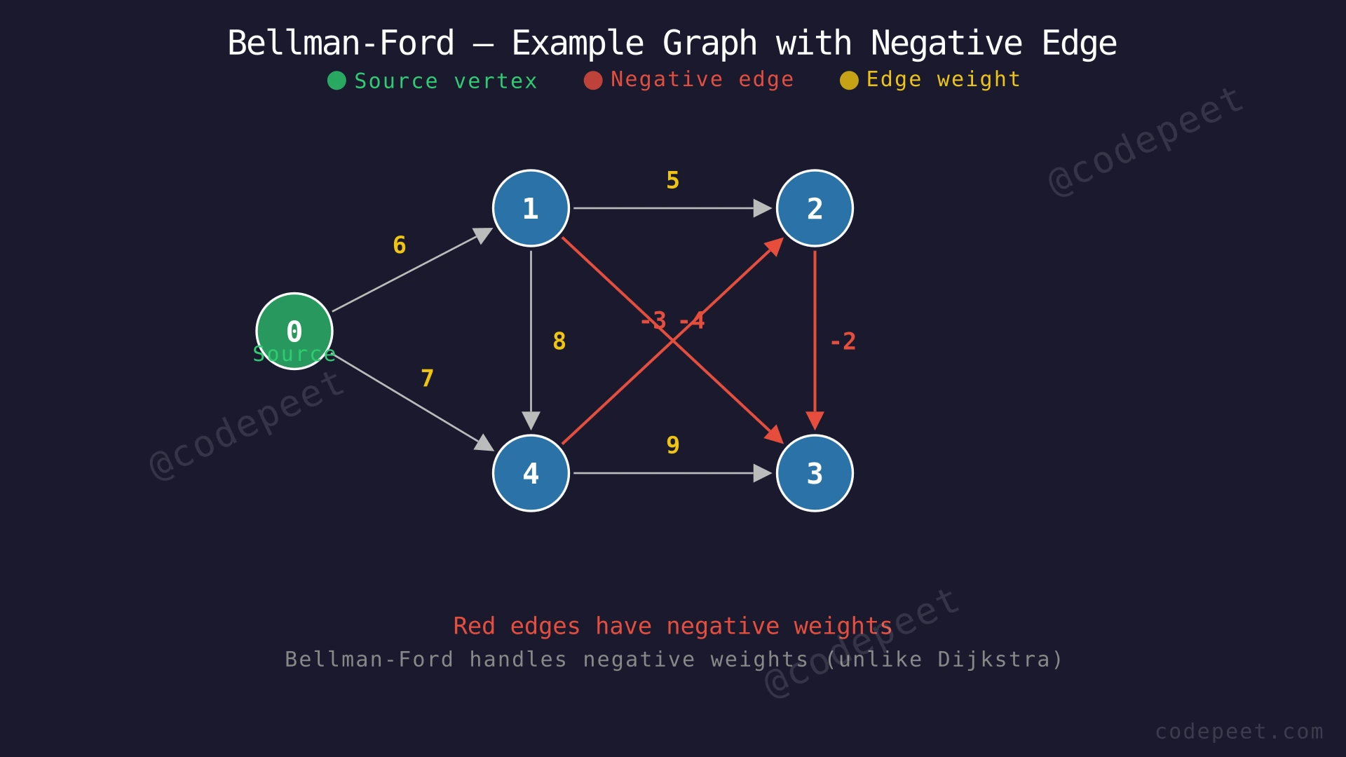
Bellman-Ford — Edge Relaxation Across Iterations — Watch how the algorithm relaxes edges iteration by iteration, propagating shortest-path information outward from the source. The negative edge 4→3 improves vertex 3's distance below what a positive-only path provides.
Algorithm
- Create a distance array of size V. Initialize all values to 10^8 (infinity), except dist[src] = 0.
- Repeat the following V-1 times (or until no updates occur in an iteration):
- For each edge (u, v, w) in the edge list:
- If dist[u] ≠ ∞ and dist[u] + w < dist[v], then update dist[v] = dist[u] + w.
- This is called relaxation of the edge.
- For each edge (u, v, w) in the edge list:
- Negative cycle detection: After V-1 iterations, perform one additional pass over all edges:
- If any edge (u, v, w) satisfies dist[u] + w < dist[v], a negative weight cycle exists.
- Return [-1] in this case.
- If no negative cycle is found, return the distance array.
Why V-1 iterations suffice: A shortest simple path has at most V-1 edges. In each iteration, the correct shortest distance "propagates" at least one edge further from the source. After V-1 iterations, all shortest distances are finalized.
Code
#include <vector>
using namespace std;

class Solution {
public:
    vector<int> bellmanFord(int V, vector<vector<int>>& edges, int src) {
        vector<int> dist(V, 1e8);
        dist[src] = 0;

        // Relax all edges V-1 times
        for (int i = 0; i < V - 1; i++) {
            bool updated = false;
            for (auto& edge : edges) {
                int u = edge[0], v = edge[1], w = edge[2];
                if (dist[u] != (int)1e8 && dist[u] + w < dist[v]) {
                    dist[v] = dist[u] + w;
                    updated = true;
                }
            }
            // Early stop: if no update happened, distances are final
            if (!updated) break;
        }

        // Check for negative weight cycle (Vth iteration)
        for (auto& edge : edges) {
            int u = edge[0], v = edge[1], w = edge[2];
            if (dist[u] != (int)1e8 && dist[u] + w < dist[v]) {
                return {-1};
            }
        }

        return dist;
    }
};
class Solution:
def bellmanFord(self, V, edges, src):
dist = [10**8] * V
dist[src] = 0
# Relax all edges V-1 times
for i in range(V - 1):
updated = False
for u, v, w in edges:
if dist[u] != 10**8 and dist[u] + w < dist[v]:
dist[v] = dist[u] + w
updated = True
# Early stop: if no update happened, distances are final
if not updated:
break
# Check for negative weight cycle (Vth iteration)
for u, v, w in edges:
if dist[u] != 10**8 and dist[u] + w < dist[v]:
return [-1]
return distimport java.util.*;
class Solution {
public int[] bellmanFord(int V, int[][] edges, int src) {
int[] dist = new int[V];
Arrays.fill(dist, (int)1e8);
dist[src] = 0;
// Relax all edges V-1 times
for (int i = 0; i < V - 1; i++) {
boolean updated = false;
for (int[] edge : edges) {
int u = edge[0], v = edge[1], w = edge[2];
if (dist[u] != (int)1e8 && dist[u] + w < dist[v]) {
dist[v] = dist[u] + w;
updated = true;
}
}
// Early stop: if no update happened, distances are final
if (!updated) break;
}
// Check for negative weight cycle (Vth iteration)
for (int[] edge : edges) {
int u = edge[0], v = edge[1], w = edge[2];
if (dist[u] != (int)1e8 && dist[u] + w < dist[v]) {
return new int[]{-1};
}
}
return dist;
}
}Complexity Analysis
Time Complexity: O(V × E)
The algorithm runs at most V-1 iterations (the outer loop). In each iteration, it scans through all E edges and performs a constant-time relaxation check for each edge. The total work is therefore (V-1) × E = O(V × E).
With the early-stop optimization (halting when no updates occur in an iteration), the algorithm often finishes in fewer than V-1 iterations. However, the worst case remains O(V × E).
For the given constraints (V ≤ 500, E ≤ V²), the worst case is approximately 500 × 250,000 = 1.25 × 10^8 operations, which is feasible within typical time limits.
Space Complexity: O(V)
We store a distance array of size V. The edge list is provided as input and does not count as additional space. No other data structures that grow with input size are used.