Unique Paths II
Description
You are given an m × n grid where a robot starts at the top-left corner (position grid[0][0]) and wants to reach the bottom-right corner (position grid[m-1][n-1]).
The robot can only move in two directions at any point in time:
- Down — moving to the next row
- Right — moving to the next column
The grid contains obstacles and empty spaces:
- A cell with value 0 represents an empty space the robot can walk through
- A cell with value 1 represents an obstacle that blocks the robot's path
The robot cannot step on or pass through any obstacle. Return the total number of unique paths from the top-left corner to the bottom-right corner. If no valid path exists (because obstacles block every possible route), return 0.
Examples
Example 1
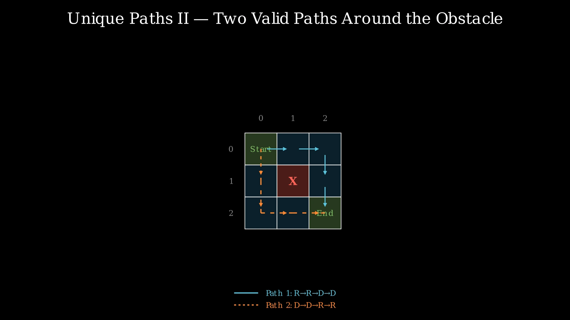
Input: obstacleGrid = [[0,0,0],[0,1,0],[0,0,0]]
Output: 2
Explanation: There is one obstacle in the center of the 3×3 grid at position (1,1). The robot must navigate around it. There are exactly two valid paths:
- Right → Right → Down → Down (go along the top, then down the right side)
- Down → Down → Right → Right (go down the left side, then along the bottom)
Any path that tries to go through the center cell (1,1) is blocked by the obstacle.
Example 2
Input: obstacleGrid = [[0,1],[0,0]]
Output: 1
Explanation: The grid is 2×2 with an obstacle at position (0,1). The robot cannot go right from (0,0) because (0,1) is blocked. The only option is to go down to (1,0), then right to (1,1). So there is exactly 1 unique path: Down → Right.
Example 3
Input: obstacleGrid = [[1,0]]
Output: 0
Explanation: The starting cell (0,0) itself is an obstacle. The robot cannot even begin its journey, so there are 0 valid paths.
Constraints
- m == obstacleGrid.length
- n == obstacleGrid[i].length
- 1 ≤ m, n ≤ 100
- obstacleGrid[i][j] is 0 or 1
- The answer will be less than or equal to 2 × 10^9
Editorial
Brute Force
Intuition
The most natural way to think about this problem is to simulate the robot's journey. At every cell, the robot has at most two choices: move right or move down. We can explore every possible combination of moves using recursion.
Imagine standing at a crossroads where you can only go east or south. At every intersection you reach, you fork into two copies of yourself — one going east, one going south. Eventually, some copies reach the destination, some hit walls (obstacles or grid boundaries), and some walk off the map. Count how many copies made it to the destination — that is your answer.
Define a function dfs(i, j) that returns the number of unique paths from cell (i, j) to the bottom-right corner. The base cases are:
- If (i, j) is out of bounds or is an obstacle → return 0
- If (i, j) is the destination (m-1, n-1) → return 1
The recursive case: dfs(i, j) = dfs(i+1, j) + dfs(i, j+1) — the total paths from here equals the paths going down plus the paths going right.
Without any memoization, this recursion re-explores the same cells from different paths, leading to an exponential number of calls.
Step-by-Step Explanation
Let's trace through with obstacleGrid = [[0,0,0],[0,1,0],[0,0,0]] (3×3 grid with obstacle at (1,1)):
Step 1: Call dfs(0,0). Not out of bounds, not an obstacle, not the destination. Recurse: dfs(1,0) + dfs(0,1).
Step 2: Explore dfs(1,0) — go down from (0,0). Cell (1,0) is empty. Recurse: dfs(2,0) + dfs(1,1).
Step 3: Explore dfs(2,0) — go down from (1,0). Cell (2,0) is empty. Recurse: dfs(3,0) + dfs(2,1).
Step 4: dfs(3,0) returns 0 — row 3 is out of bounds.
Step 5: Explore dfs(2,1) — go right from (2,0). Cell (2,1) is empty. Recurse: dfs(3,1) + dfs(2,2).
Step 6: dfs(3,1) returns 0 — out of bounds. dfs(2,2) returns 1 — destination reached! So dfs(2,1) = 0 + 1 = 1.
Step 7: Back to dfs(2,0) = dfs(3,0) + dfs(2,1) = 0 + 1 = 1.
Step 8: Explore dfs(1,1) — go right from (1,0). Cell (1,1) is an OBSTACLE! Return 0 immediately.
Step 9: Back to dfs(1,0) = dfs(2,0) + dfs(1,1) = 1 + 0 = 1. One path goes down the left side.
Step 10: Now explore dfs(0,1) — go right from (0,0). Cell (0,1) is empty. Recurse: dfs(1,1) + dfs(0,2).
Step 11: dfs(1,1) = 0 again — obstacle! This is a REPEATED computation (same cell explored again from a different path).
Step 12: Explore dfs(0,2) — go right from (0,1). Recurse: dfs(1,2) + dfs(0,3). dfs(0,3) = 0 (out of bounds).
Step 13: Explore dfs(1,2). Recurse: dfs(2,2) + dfs(1,3). dfs(2,2) = 1 (destination — also a REPEATED computation!). dfs(1,3) = 0 (out of bounds). So dfs(1,2) = 1.
Step 14: dfs(0,2) = 1 + 0 = 1. dfs(0,1) = 0 + 1 = 1.
Step 15: Final answer: dfs(0,0) = dfs(1,0) + dfs(0,1) = 1 + 1 = 2.
Unique Paths II — Recursive Exploration for 3×3 Grid — Watch how the recursion explores all possible paths, hitting obstacles and grid boundaries. Notice cells like (1,1) and (2,2) are computed more than once — overlapping subproblems.
Algorithm
- Define dfs(i, j) = number of unique paths from (i, j) to (m-1, n-1)
- Base cases:
- If i ≥ m or j ≥ n → return 0 (out of bounds)
- If obstacleGrid[i][j] == 1 → return 0 (obstacle)
- If i == m-1 and j == n-1 → return 1 (destination reached)
- Recursive case: dfs(i, j) = dfs(i+1, j) + dfs(i, j+1)
- Return dfs(0, 0)
Code
class Solution {
public:
    int uniquePathsWithObstacles(vector<vector<int>>& obstacleGrid) {
        int m = obstacleGrid.size();
        int n = obstacleGrid[0].size();

        function<int(int, int)> dfs = [&](int i, int j) -> int {
            if (i >= m || j >= n || obstacleGrid[i][j] == 1)
                return 0;
            if (i == m - 1 && j == n - 1)
                return 1;
            return dfs(i + 1, j) + dfs(i, j + 1);
        };

        return dfs(0, 0);
    }
};
class Solution:
def uniquePathsWithObstacles(self, obstacleGrid: list[list[int]]) -> int:
m, n = len(obstacleGrid), len(obstacleGrid[0])
def dfs(i: int, j: int) -> int:
if i >= m or j >= n or obstacleGrid[i][j] == 1:
return 0
if i == m - 1 and j == n - 1:
return 1
return dfs(i + 1, j) + dfs(i, j + 1)
return dfs(0, 0)class Solution {
private int[][] grid;
private int m, n;
public int uniquePathsWithObstacles(int[][] obstacleGrid) {
this.grid = obstacleGrid;
this.m = obstacleGrid.length;
this.n = obstacleGrid[0].length;
return dfs(0, 0);
}
private int dfs(int i, int j) {
if (i >= m || j >= n || grid[i][j] == 1)
return 0;
if (i == m - 1 && j == n - 1)
return 1;
return dfs(i + 1, j) + dfs(i, j + 1);
}
}Complexity Analysis
Time Complexity: O(2^(m+n))
At each cell, the recursion branches into two sub-calls (down and right). The longest path from (0,0) to (m-1,n-1) takes m+n-2 steps. Without memoization, many cells are visited repeatedly from different paths, leading to an exponential number of total calls. In the worst case (no obstacles, all cells reachable), the recursion tree has depth m+n-2 and branching factor 2.
Space Complexity: O(m + n)
The maximum recursion depth is m+n-2 (the length of the longest path from start to destination), so the call stack uses O(m+n) space.
Why This Approach Is Not Efficient
The brute force has O(2^(m+n)) time complexity, which is catastrophic for the constraint m, n ≤ 100. For a 100×100 grid, 2^198 ≈ 10^59 — far beyond any computer's capability.
The root cause is overlapping subproblems. The function dfs(i, j) gets called multiple times for the same cell (i, j) from different paths. In our 3×3 example, dfs(1,1) and dfs(2,2) were each computed twice. In larger grids, cells near the center can be reached from exponentially many different paths, each triggering a fresh computation.
Since dfs(i, j) depends only on the position (i, j) — not on how we arrived there — there are only m×n distinct subproblems. By caching results, we can ensure each cell is computed exactly once, reducing time from O(2^(m+n)) to O(m×n).
Better Approach - Top-Down DP (Memoized Recursion)
Intuition
The brute force recursion was correct but slow because it recomputed dfs(i, j) for the same cell many times. The fix is simple: add a cache. Before computing dfs(i, j), check if we already have the answer. If yes, return it immediately. If no, compute it, store the result, and return.
This is called memoization or top-down dynamic programming. We keep the natural recursive structure of the solution but add a lookup table to avoid redundant work.
The recurrence is unchanged:
- dfs(i, j) = dfs(i+1, j) + dfs(i, j+1)
- With obstacles: if obstacleGrid[i][j] == 1, then dfs(i, j) = 0
With memoization, each of the m×n cells is computed exactly once. Each computation does constant work (one addition, two lookups). Total time: O(m×n).
Step-by-Step Explanation
Let's trace through with obstacleGrid = [[0,0,0],[0,1,0],[0,0,0]] using memoization:
Step 1: Call dfs(0,0). Not in cache. Need dfs(1,0) and dfs(0,1). Start with dfs(1,0).
Step 2: dfs(1,0) not in cache. Need dfs(2,0) and dfs(1,1).
Step 3: dfs(2,0) not in cache. Need dfs(3,0) and dfs(2,1). dfs(3,0)=0 (out of bounds).
Step 4: dfs(2,1) not in cache. Need dfs(3,1) and dfs(2,2). dfs(3,1)=0 (out of bounds). dfs(2,2)=1 (destination). Cache: dfs(2,2)=1. dfs(2,1)=0+1=1. Cache: dfs(2,1)=1.
Step 5: Back to dfs(2,0)=0+1=1. Cache: dfs(2,0)=1.
Step 6: dfs(1,1): obstacle! Return 0. Cache: dfs(1,1)=0.
Step 7: dfs(1,0)=1+0=1. Cache: dfs(1,0)=1.
Step 8: Now dfs(0,1). Need dfs(1,1) and dfs(0,2). dfs(1,1) is IN CACHE → return 0 instantly! No recomputation.
Step 9: dfs(0,2) not in cache. Need dfs(1,2) and dfs(0,3). dfs(0,3)=0 (out of bounds).
Step 10: dfs(1,2) not in cache. Need dfs(2,2) and dfs(1,3). dfs(2,2) is IN CACHE → return 1 instantly! dfs(1,3)=0. dfs(1,2)=1+0=1. Cache: dfs(1,2)=1.
Step 11: dfs(0,2)=1+0=1. Cache: dfs(0,2)=1.
Step 12: dfs(0,1)=0+1=1. Cache: dfs(0,1)=1.
Step 13: dfs(0,0)=dfs(1,0)+dfs(0,1)=1+1=2. Answer: 2!
Unique Paths II — Memoized DP Table for 3×3 Grid — Watch how the memo cache fills as the recursion explores cells. Cached lookups (highlighted) avoid recomputation of overlapping subproblems.
Algorithm
- Create a memo table (or use @cache decorator) for m×n cells
- Define dfs(i, j) with memoization:
- If i ≥ m or j ≥ n or obstacleGrid[i][j] == 1 → return 0
- If i == m-1 and j == n-1 → return 1
- If (i, j) is in cache → return cached value
- Compute result = dfs(i+1, j) + dfs(i, j+1)
- Store result in cache and return
- Return dfs(0, 0)
Code
class Solution {
public:
    int uniquePathsWithObstacles(vector<vector<int>>& obstacleGrid) {
        int m = obstacleGrid.size();
        int n = obstacleGrid[0].size();
        vector<vector<int>> memo(m, vector<int>(n, -1));

        function<int(int, int)> dfs = [&](int i, int j) -> int {
            if (i >= m || j >= n || obstacleGrid[i][j] == 1)
                return 0;
            if (i == m - 1 && j == n - 1)
                return 1;
            if (memo[i][j] != -1)
                return memo[i][j];
            return memo[i][j] = dfs(i + 1, j) + dfs(i, j + 1);
        };

        return dfs(0, 0);
    }
};
from functools import cache
class Solution:
def uniquePathsWithObstacles(self, obstacleGrid: list[list[int]]) -> int:
m, n = len(obstacleGrid), len(obstacleGrid[0])
@cache
def dfs(i: int, j: int) -> int:
if i >= m or j >= n or obstacleGrid[i][j] == 1:
return 0
if i == m - 1 and j == n - 1:
return 1
return dfs(i + 1, j) + dfs(i, j + 1)
return dfs(0, 0)class Solution {
private int[][] grid;
private int m, n;
private Integer[][] memo;
public int uniquePathsWithObstacles(int[][] obstacleGrid) {
this.grid = obstacleGrid;
this.m = obstacleGrid.length;
this.n = obstacleGrid[0].length;
this.memo = new Integer[m][n];
return dfs(0, 0);
}
private int dfs(int i, int j) {
if (i >= m || j >= n || grid[i][j] == 1)
return 0;
if (i == m - 1 && j == n - 1)
return 1;
if (memo[i][j] != null)
return memo[i][j];
return memo[i][j] = dfs(i + 1, j) + dfs(i, j + 1);
}
}Complexity Analysis
Time Complexity: O(m × n)
There are m×n unique cells in the grid. Each cell is computed exactly once due to memoization. For each cell, we do O(1) work (one addition, two cache lookups). Total: m×n × O(1) = O(m×n).
Space Complexity: O(m × n)
The memo table stores results for up to m×n cells, using O(m×n) space. Additionally, the recursion stack can go as deep as m+n-2 in the worst case (the longest path length), using O(m+n) space. Since m×n dominates m+n, the total space is O(m×n).
Why This Approach Is Not Efficient
The memoized recursion achieves O(m×n) time, which is already optimal — we must examine each cell at least once. However, there are two practical concerns:
-
Recursion stack depth: The recursion can go as deep as m+n-2. For a 100×100 grid, that is 198 levels deep. While manageable in C++ and Java, Python's default recursion limit of 1000 could be exceeded for larger grids, causing a RecursionError.
-
Space usage: The memo table requires O(m×n) space. We can observe that when filling the DP table bottom-up (iteratively), each row only depends on the row below it. This means we can optimize space from O(m×n) to O(n) by using a single 1D array that we update row by row.
The bottom-up iterative approach eliminates the recursion stack entirely and reduces space from O(m×n) to O(n), making it more memory-efficient and safer for large inputs.
Optimal Approach - Bottom-Up DP with Space Optimization
Intuition
Instead of computing the DP table recursively, we fill it iteratively from top-left to bottom-right. Define dp[i][j] as the number of unique paths from the start (0,0) to cell (i,j). The recurrence is:
- dp[0][0] = 1 (if start is not an obstacle)
- For the first row: dp[0][j] = dp[0][j-1] if no obstacle, else 0
- For the first column: dp[i][0] = dp[i-1][0] if no obstacle, else 0
- For all other cells: dp[i][j] = dp[i-1][j] + dp[i][j-1] if no obstacle, else 0
The key space optimization: since dp[i][j] only depends on dp[i-1][j] (the cell directly above) and dp[i][j-1] (the cell to the left), we only need the current row as we process it left-to-right. We reuse a single 1D array dp[j] where:
- Before updating dp[j] for the current row, dp[j] still holds the value from the previous row (which is dp[i-1][j])
- dp[j-1] has already been updated for the current row (which is dp[i][j-1])
So dp[j] = dp[j] + dp[j-1] naturally computes the correct value using the two dependencies. If the cell is an obstacle, we simply set dp[j] = 0.
This reduces space from O(m×n) to O(n) while maintaining O(m×n) time.
Step-by-Step Explanation
Let's trace through with obstacleGrid = [[0,0,0],[0,1,0],[0,0,0]] using the 1D DP array:
Step 1: Initialize dp array for the first row. Process each cell left-to-right.
- dp[0]: grid[0][0]=0 (empty), set dp[0]=1 (start cell)
- dp = [1, ?, ?]
Step 2: dp[1]: grid[0][1]=0 (empty), dp[1] = dp[0] = 1 (can reach from left)
- dp = [1, 1, ?]
Step 3: dp[2]: grid[0][2]=0 (empty), dp[2] = dp[1] = 1 (can reach from left)
- dp = [1, 1, 1]
Step 4: Now process row 1. dp[0]: grid[1][0]=0 (empty). dp[0] stays dp[0]=1 (can reach from above). dp = [1, 1, 1]
Step 5: dp[1]: grid[1][1]=1 — OBSTACLE! Set dp[1]=0. No paths go through an obstacle.
- dp = [1, 0, 1]
Step 6: dp[2]: grid[1][2]=0 (empty). dp[2] = dp[2](from above) + dp[1](from left) = 1 + 0 = 1.
- dp = [1, 0, 1]
Step 7: Process row 2. dp[0]: grid[2][0]=0 (empty). dp[0] stays 1 (from above).
- dp = [1, 0, 1]
Step 8: dp[1]: grid[2][1]=0 (empty). dp[1] = dp[1](from above=0) + dp[0](from left=1) = 0 + 1 = 1.
- dp = [1, 1, 1]
Step 9: dp[2]: grid[2][2]=0 (empty). dp[2] = dp[2](from above=1) + dp[1](from left=1) = 1 + 1 = 2.
- dp = [1, 1, 2]
Step 10: Answer: dp[n-1] = dp[2] = 2.
Unique Paths II — 1D DP Array Row-by-Row Update — Watch how a single 1D array is reused for each row. Before update, dp[j] holds the value from the row above. After update, it holds the current row's value.
Algorithm
- If the start cell or destination cell is an obstacle, return 0
- Create a 1D array dp of size n, initialized to 0
- Set dp[0] = 1 (one way to reach the start)
- For the first row, fill dp[j] = dp[j-1] if grid[0][j] == 0, else dp[j] = 0
- For each subsequent row i from 1 to m-1:
- If grid[i][0] == 1, set dp[0] = 0 (obstacle in first column blocks all paths below)
- For each column j from 1 to n-1:
- If grid[i][j] == 1: dp[j] = 0
- Else: dp[j] = dp[j] + dp[j-1] (paths from above + paths from left)
- Return dp[n-1]
Code
class Solution {
public:
    int uniquePathsWithObstacles(vector<vector<int>>& obstacleGrid) {
        int m = obstacleGrid.size();
        int n = obstacleGrid[0].size();

        if (obstacleGrid[0][0] == 1 || obstacleGrid[m-1][n-1] == 1)
            return 0;

        vector<int> dp(n, 0);
        dp[0] = 1;

        for (int i = 0; i < m; i++) {
            for (int j = 0; j < n; j++) {
                if (obstacleGrid[i][j] == 1) {
                    dp[j] = 0;
                } else if (j > 0) {
                    dp[j] += dp[j - 1];
                }
                // If j == 0 and no obstacle, dp[j] keeps
                // its value from the row above (unchanged)
            }
        }

        return dp[n - 1];
    }
};
class Solution:
def uniquePathsWithObstacles(self, obstacleGrid: list[list[int]]) -> int:
m, n = len(obstacleGrid), len(obstacleGrid[0])
if obstacleGrid[0][0] == 1 or obstacleGrid[m-1][n-1] == 1:
return 0
dp = [0] * n
dp[0] = 1
for i in range(m):
for j in range(n):
if obstacleGrid[i][j] == 1:
dp[j] = 0
elif j > 0:
dp[j] += dp[j - 1]
# If j == 0 and no obstacle, dp[j] keeps
# its value from the row above (unchanged)
return dp[n - 1]class Solution {
public int uniquePathsWithObstacles(int[][] obstacleGrid) {
int m = obstacleGrid.length;
int n = obstacleGrid[0].length;
if (obstacleGrid[0][0] == 1 || obstacleGrid[m-1][n-1] == 1)
return 0;
int[] dp = new int[n];
dp[0] = 1;
for (int i = 0; i < m; i++) {
for (int j = 0; j < n; j++) {
if (obstacleGrid[i][j] == 1) {
dp[j] = 0;
} else if (j > 0) {
dp[j] += dp[j - 1];
}
// If j == 0 and no obstacle, dp[j] keeps
// its value from the row above (unchanged)
}
}
return dp[n - 1];
}
}Complexity Analysis
Time Complexity: O(m × n)
We iterate through every cell of the m×n grid exactly once. For each cell, we do O(1) work (one comparison, one addition, one assignment). Total: m × n × O(1) = O(m×n). This is optimal since we must read every cell to check for obstacles.
Space Complexity: O(n)
We use a single 1D array of size n, which stores the DP values for the current row being processed. No recursion stack is used (iterative approach). This is a significant improvement over the O(m×n) space of the memoized approach, especially for large grids like 100×100 where we reduce from 10,000 cells of storage to just 100.