Shortest Path in DAG
Description
Given a Directed Acyclic Graph (DAG) with V vertices numbered from 0 to V-1 and E weighted directed edges, find the shortest path from the source vertex 0 to every other vertex.
You are given:
V: the number of verticesE: the number of edgesedges[][]: a 2D array where each entry[u, v, w]represents a directed edge from vertexuto vertexvwith weightw
Return an array dist[] of size V where dist[i] is the shortest distance from vertex 0 to vertex i. If a vertex is unreachable from the source, its distance should be -1.
A DAG is a directed graph with no cycles — you can never start at a vertex and follow directed edges to return to the same vertex. This special property allows us to find shortest paths more efficiently than in general graphs.
Examples
Example 1
Input: V = 4, E = 2, edges = [[0,1,2], [0,2,1]]
Graph:
0 ---(2)---> 1
0 ---(1)---> 2
(vertex 3 has no incoming or outgoing edges from source)
Output: [0, 2, 1, -1]
Explanation:
- dist[0] = 0 (source vertex, distance to itself is 0)
- dist[1] = 2 (direct edge 0→1 with weight 2)
- dist[2] = 1 (direct edge 0→2 with weight 1)
- dist[3] = -1 (vertex 3 is unreachable — no path exists from vertex 0 to vertex 3)
Example 2
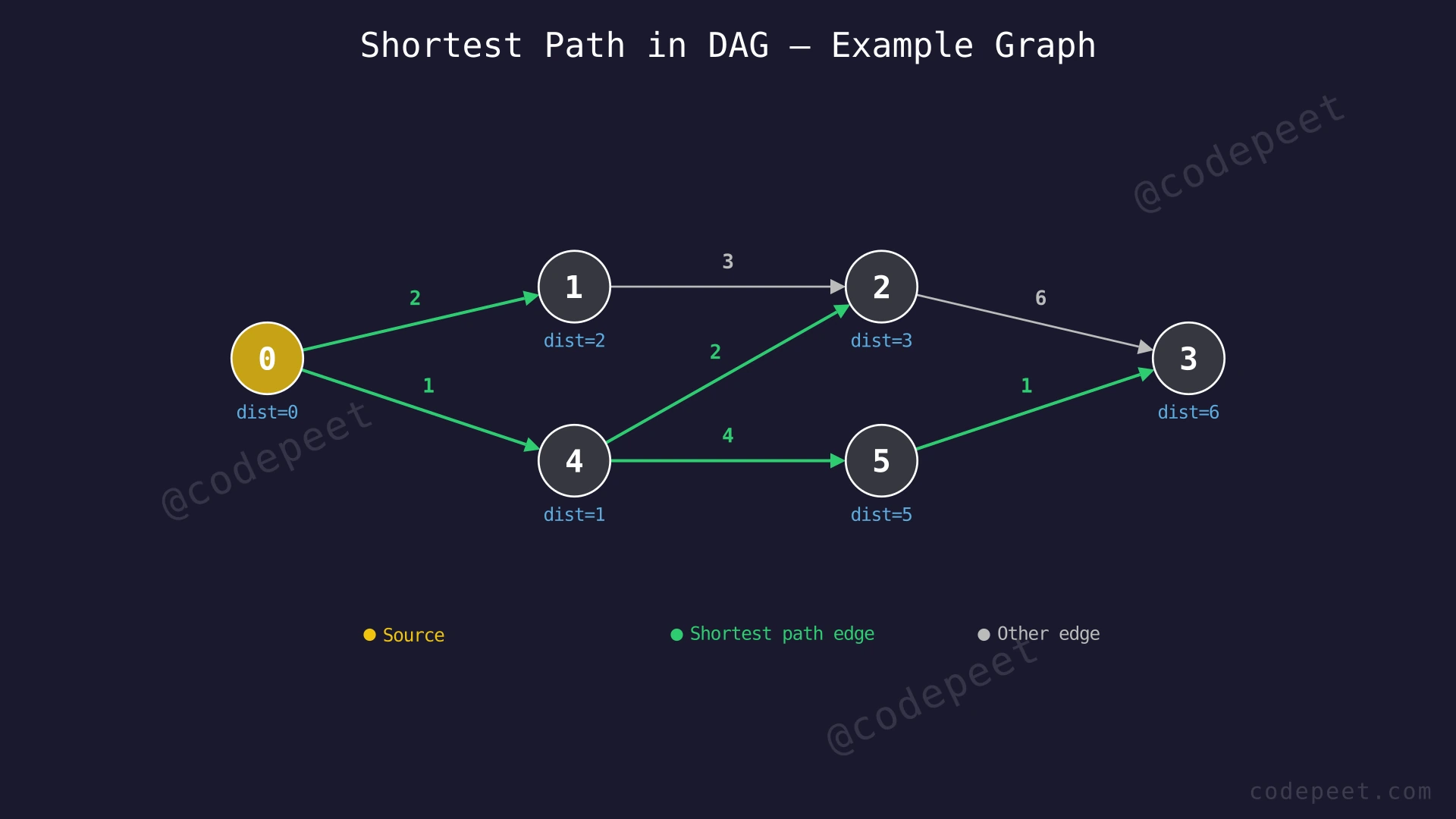
Input: V = 6, E = 7, edges = [[0,1,2], [0,4,1], [4,5,4], [4,2,2], [1,2,3], [2,3,6], [5,3,1]]
Graph:
0 ---(2)---> 1 ---(3)---> 2 ---(6)---> 3
|                          ^              ^
|---(1)---> 4 ---(2)------+              |
            |                             |
            +---(4)---> 5 ---(1)----------+
Output: [0, 2, 3, 6, 1, 5]
Explanation:
- dist[0] = 0 (source)
- dist[1] = 2 (path: 0→1, weight 2)
- dist[2] = 3 (path: 0→4→2, weight 1+2=3. Note: 0→1→2 costs 2+3=5 which is longer)
- dist[3] = 6 (path: 0→4→5→3, weight 1+4+1=6. Note: 0→4→2→3 costs 1+2+6=9, and 0→1→2→3 costs 2+3+6=11, both longer)
- dist[4] = 1 (path: 0→4, weight 1)
- dist[5] = 5 (path: 0→4→5, weight 1+4=5)
Example 3
Input: V = 3, E = 3, edges = [[0,1,1], [0,2,10], [1,2,3]]
Output: [0, 1, 4]
Explanation:
- dist[0] = 0 (source)
- dist[1] = 1 (direct edge 0→1 with weight 1)
- dist[2] = 4 (path: 0→1→2, weight 1+3=4. The direct edge 0→2 costs 10 which is longer. The indirect path through vertex 1 is cheaper.)
Constraints
- 1 ≤ V ≤ 100
- 1 ≤ E ≤ min(V × (V-1) / 2, 4000)
- 0 ≤ edges[i][0], edges[i][1] < V
- 0 ≤ edges[i][2] ≤ 10^5
- The graph is a Directed Acyclic Graph (no cycles)
Editorial
Brute Force
Intuition
The most natural way to find the shortest path from source to every vertex is to enumerate all possible paths using DFS and track the minimum cost for each destination.
Think of it like exploring a road network. You're at city 0 and want to find the cheapest route to every other city. The brute-force approach is like a traveler who explores every possible route — taking every fork in the road, recording the cost, and at the end comparing all routes to each destination to find the cheapest one.
Since the graph is a DAG (no cycles), the DFS will always terminate — you can never loop back to a city you've already visited on the current path. However, you might visit the same city multiple times through different paths, and each time you reach it with a lower cost, you explore all its outgoing edges again.
The key problem: if vertex X has many incoming paths, you end up re-exploring all edges from X multiple times. This leads to exponential work in the worst case.
Step-by-Step Explanation
Let's trace with V = 6, E = 7, edges = [[0,1,2],[0,4,1],[4,5,4],[4,2,2],[1,2,3],[2,3,6],[5,3,1]].
We want to find shortest paths from vertex 0 to all vertices. We use DFS from source, exploring all outgoing edges and updating distances whenever we find a shorter path.
Step 1: Initialize dist = [0, ∞, ∞, ∞, ∞, ∞]. Start DFS from vertex 0 with cost 0.
Step 2: At vertex 0 (cost=0). Explore edge 0→1 (weight 2). New cost = 0+2 = 2 < ∞. Update dist[1] = 2. Recurse into vertex 1.
Step 3: At vertex 1 (cost=2). Explore edge 1→2 (weight 3). New cost = 2+3 = 5 < ∞. Update dist[2] = 5. Recurse into vertex 2.
Step 4: At vertex 2 (cost=5). Explore edge 2→3 (weight 6). New cost = 5+6 = 11 < ∞. Update dist[3] = 11. Recurse into vertex 3.
Step 5: At vertex 3 (cost=11). No outgoing edges. Backtrack to vertex 2, then to vertex 1, then to vertex 0.
Step 6: Back at vertex 0. Explore edge 0→4 (weight 1). New cost = 0+1 = 1 < ∞. Update dist[4] = 1. Recurse into vertex 4.
Step 7: At vertex 4 (cost=1). Explore edge 4→5 (weight 4). New cost = 1+4 = 5 < ∞. Update dist[5] = 5. Recurse into vertex 5.
Step 8: At vertex 5 (cost=5). Explore edge 5→3 (weight 1). New cost = 5+1 = 6 < 11. Update dist[3] = 6 (improved!). Recurse into vertex 3.
Step 9: At vertex 3 (cost=6). No outgoing edges. Backtrack to vertex 5, then to vertex 4.
Step 10: At vertex 4. Explore edge 4→2 (weight 2). New cost = 1+2 = 3 < 5. Update dist[2] = 3 (improved!). Recurse into vertex 2.
Step 11: At vertex 2 (cost=3). Explore edge 2→3 (weight 6). New cost = 3+6 = 9 > 6. No improvement. Don't recurse.
Step 12: All paths explored. Final dist = [0, 2, 3, 6, 1, 5]. Replace ∞ with -1 for unreachable vertices.
Result: [0, 2, 3, 6, 1, 5]
DFS All Paths — Exploring Every Route from Source — Watch DFS explore every possible path from vertex 0, updating shortest distances whenever a cheaper route is found. Notice how vertex 3 is visited twice as better paths are discovered.
Algorithm
- Build an adjacency list from the edges array.
- Initialize
dist[]with ∞ for all vertices. Setdist[source] = 0. - Define a recursive DFS function
dfs(u, cost):
a. For each neighborvofuwith edge weightw:- If
cost + w < dist[v]:- Update
dist[v] = cost + w - Recursively call
dfs(v, cost + w)
- Update
- If
- Call
dfs(source, 0)to start the exploration. - Replace any remaining ∞ values with -1 (unreachable vertices).
- Return
dist[].
Code
class Solution {
public:
    void dfs(int u, int cost, vector<vector<pair<int,int>>>& adj, vector<int>& dist) {
        for (auto& [v, w] : adj[u]) {
            if (cost + w < dist[v]) {
                dist[v] = cost + w;
                dfs(v, cost + w, adj, dist);
            }
        }
    }

    vector<int> shortestPath(int V, int E, vector<vector<int>>& edges) {
        vector<vector<pair<int,int>>> adj(V);
        for (auto& e : edges) {
            adj[e[0]].push_back({e[1], e[2]});
        }

        vector<int> dist(V, INT_MAX);
        dist[0] = 0;
        dfs(0, 0, adj, dist);

        for (int i = 0; i < V; i++) {
            if (dist[i] == INT_MAX) dist[i] = -1;
        }
        return dist;
    }
};
class Solution:
def shortestPath(self, V, E, edges):
adj = [[] for _ in range(V)]
for u, v, w in edges:
adj[u].append((v, w))
dist = [float('inf')] * V
dist[0] = 0
def dfs(u, cost):
for v, w in adj[u]:
if cost + w < dist[v]:
dist[v] = cost + w
dfs(v, cost + w)
dfs(0, 0)
return [d if d != float('inf') else -1 for d in dist]class Solution {
public int[] shortestPath(int V, int E, int[][] edges) {
List<List<int[]>> adj = new ArrayList<>();
for (int i = 0; i < V; i++) adj.add(new ArrayList<>());
for (int[] e : edges) {
adj.get(e[0]).add(new int[]{e[1], e[2]});
}
int[] dist = new int[V];
Arrays.fill(dist, Integer.MAX_VALUE);
dist[0] = 0;
dfs(0, 0, adj, dist);
for (int i = 0; i < V; i++) {
if (dist[i] == Integer.MAX_VALUE) dist[i] = -1;
}
return dist;
}
private void dfs(int u, int cost, List<List<int[]>> adj, int[] dist) {
for (int[] edge : adj.get(u)) {
int v = edge[0], w = edge[1];
if (cost + w < dist[v]) {
dist[v] = cost + w;
dfs(v, cost + w, adj, dist);
}
}
}
}Complexity Analysis
Time Complexity: O(V × 2^V) in the worst case
In a DAG, the number of distinct paths from source to any vertex can be exponential. Consider a layered DAG where each vertex in layer i connects to every vertex in layer i+1. The number of paths grows exponentially with the number of layers. Each time we discover a shorter path to a vertex, we re-explore all its outgoing edges, potentially triggering a cascade of re-explorations.
For the given constraints (V ≤ 100), this can lead to an enormous number of path explorations in adversarial inputs.
Space Complexity: O(V + E)
- O(V + E) for the adjacency list.
- O(V) for the distance array.
- O(V) for the recursion stack in the worst case (a path through all V vertices).
Why This Approach Is Not Efficient
The brute-force DFS has a critical flaw: redundant re-exploration. When we discover a shorter path to vertex X, we re-explore ALL edges from X. If X's descendants also get updated, they re-explore their edges too. This creates a cascade effect.
Consider a DAG with layers: source → layer 1 (2 nodes) → layer 2 (2 nodes) → ... → layer k (2 nodes). The number of paths from source to the last layer is 2^k. With V = 100, this means potentially 2^50 paths — far beyond any time limit.
The fundamental waste: we're processing the same vertex multiple times because we don't have a smart ordering. If we could guarantee that when we process vertex X, ALL of X's predecessors have already been finalized, we'd never need to re-explore. This insight leads to the Bellman-Ford algorithm (which bounds re-exploration to V-1 iterations) and ultimately to the topological sort approach (which processes each vertex exactly once).
Better Approach - Bellman-Ford Edge Relaxation
Intuition
Instead of following DFS paths and potentially re-exploring vertices exponentially many times, Bellman-Ford takes a systematic approach: relax every edge in the graph, and repeat this V-1 times.
"Relaxing" an edge u→v with weight w means: if dist[u] + w < dist[v], update dist[v] = dist[u] + w. In other words, check if going through u gives a shorter path to v.
Why V-1 iterations? The shortest path from source to any vertex uses at most V-1 edges (since there are V vertices and no cycles in a DAG). In the first iteration, we correctly compute distances for vertices reachable in 1 edge. In the second iteration, vertices reachable in 2 edges get their correct distances. After V-1 iterations, all vertices within V-1 edges of the source have their optimal distances.
Think of it like a ripple spreading through water. In iteration 1, the source's direct neighbors get their distances. In iteration 2, those neighbors' neighbors get correct distances. The "wavefront" advances one edge per iteration, and after V-1 iterations, it has reached every reachable vertex.
Bellman-Ford works on ANY graph (including negative weights), not just DAGs. But it's slower than necessary for DAGs because it doesn't exploit the acyclic structure.
Step-by-Step Explanation
Let's trace with V = 6, E = 7, edges = [[0,1,2],[0,4,1],[4,5,4],[4,2,2],[1,2,3],[2,3,6],[5,3,1]].
Edge list: 0→1(2), 0→4(1), 4→5(4), 4→2(2), 1→2(3), 2→3(6), 5→3(1)
Step 1: Initialize dist = [0, ∞, ∞, ∞, ∞, ∞].
Iteration 1 — Relax all 7 edges:
Step 2: Edge 0→1(2): dist[0]+2 = 0+2 = 2 < ∞. Update dist[1] = 2.
Step 3: Edge 0→4(1): dist[0]+1 = 0+1 = 1 < ∞. Update dist[4] = 1.
Step 4: Edge 4→5(4): dist[4]+4 = 1+4 = 5 < ∞. Update dist[5] = 5.
Step 5: Edge 4→2(2): dist[4]+2 = 1+2 = 3 < ∞. Update dist[2] = 3.
Step 6: Edge 1→2(3): dist[1]+3 = 2+3 = 5. But dist[2]=3 already. 5 > 3. No update.
Step 7: Edge 2→3(6): dist[2]+6 = 3+6 = 9 < ∞. Update dist[3] = 9.
Step 8: Edge 5→3(1): dist[5]+1 = 5+1 = 6 < 9. Update dist[3] = 6.
After Iteration 1: dist = [0, 2, 3, 6, 1, 5].
Iteration 2 — Relax all 7 edges again:
Step 9: Edge 0→1(2): 0+2=2, dist[1]=2. No change.
Step 10: All other edges: no changes either.
No distances changed in iteration 2 → Early termination.
Result: [0, 2, 3, 6, 1, 5]
Bellman-Ford — Systematic Edge Relaxation — Watch Bellman-Ford relax every edge in the graph one by one. Each full pass over all edges is one iteration. Distances converge to optimal values as the relaxation wavefront spreads.
Algorithm
- Build an adjacency list (or keep the edge list).
- Initialize
dist[]with ∞ for all vertices. Setdist[source] = 0. - Repeat V-1 times:
a. For each edge (u, v, w) in the edge list:- If
dist[u] ≠ ∞anddist[u] + w < dist[v]:- Update
dist[v] = dist[u] + w
b. If no distances changed in this iteration, break early.
- Update
- If
- Replace remaining ∞ values with -1.
- Return
dist[].
Code
class Solution {
public:
    vector<int> shortestPath(int V, int E, vector<vector<int>>& edges) {
        vector<int> dist(V, INT_MAX);
        dist[0] = 0;

        // Relax all edges V-1 times
        for (int iter = 0; iter < V - 1; iter++) {
            bool updated = false;
            for (auto& e : edges) {
                int u = e[0], v = e[1], w = e[2];
                if (dist[u] != INT_MAX && dist[u] + w < dist[v]) {
                    dist[v] = dist[u] + w;
                    updated = true;
                }
            }
            if (!updated) break; // Early termination
        }

        for (int i = 0; i < V; i++) {
            if (dist[i] == INT_MAX) dist[i] = -1;
        }
        return dist;
    }
};
class Solution:
def shortestPath(self, V, E, edges):
dist = [float('inf')] * V
dist[0] = 0
# Relax all edges V-1 times
for _ in range(V - 1):
updated = False
for u, v, w in edges:
if dist[u] != float('inf') and dist[u] + w < dist[v]:
dist[v] = dist[u] + w
updated = True
if not updated:
break # Early termination
return [d if d != float('inf') else -1 for d in dist]class Solution {
public int[] shortestPath(int V, int E, int[][] edges) {
int[] dist = new int[V];
Arrays.fill(dist, Integer.MAX_VALUE);
dist[0] = 0;
// Relax all edges V-1 times
for (int iter = 0; iter < V - 1; iter++) {
boolean updated = false;
for (int[] e : edges) {
int u = e[0], v = e[1], w = e[2];
if (dist[u] != Integer.MAX_VALUE && dist[u] + w < dist[v]) {
dist[v] = dist[u] + w;
updated = true;
}
}
if (!updated) break;
}
for (int i = 0; i < V; i++) {
if (dist[i] == Integer.MAX_VALUE) dist[i] = -1;
}
return dist;
}
}Complexity Analysis
Time Complexity: O(V × E)
We perform up to V-1 iterations. In each iteration, we relax all E edges. Each edge relaxation is O(1). Total: O(V × E).
With V ≤ 100 and E ≤ 4000, that's at most 400,000 operations — well within time limits. However, for larger graphs, this becomes a bottleneck.
Space Complexity: O(V)
- O(V) for the distance array.
- O(E) for the edge list (input — not additional space).
- No auxiliary data structures needed beyond the dist array.
Why This Approach Is Not Efficient
Bellman-Ford performs O(V × E) work, but for a DAG, we can do much better — O(V + E).
The inefficiency is clear: Bellman-Ford doesn't know the correct order to process vertices. It compensates by iterating over ALL edges V-1 times, hoping that each iteration propagates distances one hop further. This means edges between vertices that are already finalized get checked repeatedly for no benefit.
In our example with V=6, Bellman-Ford checked 14 edge relaxations (7 edges × 2 iterations). In the second iteration, ALL 7 checks were wasted (no updates). Across V-1=5 possible iterations, that's up to 35 total checks for a graph where only 7 are truly needed.
Key insight: A DAG has a topological order — a linear ordering where every edge goes from an earlier vertex to a later vertex. If we process vertices in this order, each vertex is processed exactly once, and when we process it, ALL paths leading to it have already been considered. This means we relax each edge exactly once, achieving O(V + E) time.
Optimal Approach - Topological Sort with Single-Pass Relaxation
Intuition
The optimal approach exploits the defining property of a DAG: it has a topological ordering. A topological order is a linear sequence of vertices where for every directed edge u→v, vertex u appears before vertex v in the sequence.
Why does this help? When we process vertex u in topological order, every vertex that could provide a shorter path TO u has already been processed. This means dist[u] is already finalized — it won't improve later. So when we relax edges from u, we're propagating a final, optimal distance.
Think of it like a factory assembly line. Each station (vertex) depends on parts from earlier stations (predecessors). If you process stations in order from start to end, each station has all its inputs ready. You never need to go back and redo anything.
The algorithm has two phases:
- Compute topological order using DFS with a stack (or Kahn's algorithm with in-degrees).
- Relax edges in topological order: for each vertex
uin the topo order, relax all outgoing edges fromu.
Each edge is relaxed exactly once, and each vertex is processed exactly once. Total time: O(V + E).
Step-by-Step Explanation
Let's trace with V = 6, E = 7, edges = [[0,1,2],[0,4,1],[4,5,4],[4,2,2],[1,2,3],[2,3,6],[5,3,1]].
Phase 1: Compute Topological Order
Using DFS-based topological sort:
Step 1: Start DFS from vertex 0. Visit 0 → 1 → 2 → 3 (dead end, push 3). Backtrack to 2 (all neighbors done, push 2). Backtrack to 1 (all done, push 1). Back to 0, visit 4 → 5 → 3 (already visited). Push 5. Back to 4, visit 2 (already visited). Push 4. Push 0.
Step 2: Stack (top to bottom): [0, 4, 1, 5, 2, 3]. Pop to get topological order: 0, 4, 1, 5, 2, 3 (or equivalently 0, 1, 4, 5, 2, 3 depending on adjacency list order).
Let's use the order: 0, 1, 4, 5, 2, 3.
Phase 2: Relax in Topological Order
Step 3: Initialize dist = [0, ∞, ∞, ∞, ∞, ∞].
Step 4: Process vertex 0 (dist[0]=0). Relax outgoing edges:
- 0→1(2): dist[1] = min(∞, 0+2) = 2. Updated!
- 0→4(1): dist[4] = min(∞, 0+1) = 1. Updated!
dist = [0, 2, ∞, ∞, 1, ∞]
Step 5: Process vertex 1 (dist[1]=2). Relax outgoing edges:
- 1→2(3): dist[2] = min(∞, 2+3) = 5. Updated!
dist = [0, 2, 5, ∞, 1, ∞]
Step 6: Process vertex 4 (dist[4]=1). Relax outgoing edges:
- 4→5(4): dist[5] = min(∞, 1+4) = 5. Updated!
- 4→2(2): dist[2] = min(5, 1+2) = 3. Updated! (improved from 5 to 3)
dist = [0, 2, 3, ∞, 1, 5]
Step 7: Process vertex 5 (dist[5]=5). Relax outgoing edges:
- 5→3(1): dist[3] = min(∞, 5+1) = 6. Updated!
dist = [0, 2, 3, 6, 1, 5]
Step 8: Process vertex 2 (dist[2]=3). Relax outgoing edges:
- 2→3(6): dist[3] = min(6, 3+6) = 6. No change! (9 > 6, path through 5 was better)
dist = [0, 2, 3, 6, 1, 5]
Step 9: Process vertex 3 (dist[3]=6). No outgoing edges.
Result: [0, 2, 3, 6, 1, 5]. Each edge relaxed exactly once. Each vertex processed exactly once.
Topological Sort + Single-Pass Relaxation — O(V+E) Shortest Paths — Watch the two-phase algorithm: first compute topological order via DFS, then relax edges in that order. Each vertex is processed exactly once, and when processed, its distance is already optimal.
Algorithm
Phase 1 — Topological Sort (DFS-based):
- Build an adjacency list from the edges.
- Create a
visited[]array and an empty stack. - For each unvisited vertex
v, run DFS:
a. Markvas visited.
b. Recursively visit all unvisited neighbors.
c. After all neighbors are done, pushvonto the stack. - Pop all elements from the stack to get the topological order.
Phase 2 — Shortest Path Relaxation:
5. Initialize dist[] with ∞ for all vertices. Set dist[source] = 0.
6. For each vertex u in topological order:
a. If dist[u] ≠ ∞ (vertex is reachable):
- For each neighbor v of u with edge weight w:
- If dist[u] + w < dist[v]:
- Update dist[v] = dist[u] + w
7. Replace remaining ∞ values with -1.
8. Return dist[].
Code
class Solution {
public:
    void topoSort(int u, vector<vector<pair<int,int>>>& adj,
                  vector<bool>& visited, stack<int>& st) {
        visited[u] = true;
        for (auto& [v, w] : adj[u]) {
            if (!visited[v]) {
                topoSort(v, adj, visited, st);
            }
        }
        st.push(u);
    }

    vector<int> shortestPath(int V, int E, vector<vector<int>>& edges) {
        // Build adjacency list
        vector<vector<pair<int,int>>> adj(V);
        for (auto& e : edges) {
            adj[e[0]].push_back({e[1], e[2]});
        }

        // Phase 1: Topological Sort
        vector<bool> visited(V, false);
        stack<int> st;
        for (int i = 0; i < V; i++) {
            if (!visited[i]) {
                topoSort(i, adj, visited, st);
            }
        }

        // Phase 2: Relax edges in topological order
        vector<int> dist(V, INT_MAX);
        dist[0] = 0;

        while (!st.empty()) {
            int u = st.top();
            st.pop();

            if (dist[u] != INT_MAX) {
                for (auto& [v, w] : adj[u]) {
                    if (dist[u] + w < dist[v]) {
                        dist[v] = dist[u] + w;
                    }
                }
            }
        }

        // Replace unreachable vertices with -1
        for (int i = 0; i < V; i++) {
            if (dist[i] == INT_MAX) dist[i] = -1;
        }
        return dist;
    }
};
import sys
from collections import defaultdict
class Solution:
def shortestPath(self, V, E, edges):
# Build adjacency list
adj = defaultdict(list)
for u, v, w in edges:
adj[u].append((v, w))
# Phase 1: Topological Sort (DFS-based)
visited = [False] * V
stack = []
def topo_dfs(u):
visited[u] = True
for v, w in adj[u]:
if not visited[v]:
topo_dfs(v)
stack.append(u)
for i in range(V):
if not visited[i]:
topo_dfs(i)
# Phase 2: Relax edges in topological order
dist = [float('inf')] * V
dist[0] = 0
while stack:
u = stack.pop()
if dist[u] != float('inf'):
for v, w in adj[u]:
if dist[u] + w < dist[v]:
dist[v] = dist[u] + w
return [d if d != float('inf') else -1 for d in dist]class Solution {
public int[] shortestPath(int V, int E, int[][] edges) {
// Build adjacency list
List<List<int[]>> adj = new ArrayList<>();
for (int i = 0; i < V; i++) adj.add(new ArrayList<>());
for (int[] e : edges) {
adj.get(e[0]).add(new int[]{e[1], e[2]});
}
// Phase 1: Topological Sort
boolean[] visited = new boolean[V];
Stack<Integer> stack = new Stack<>();
for (int i = 0; i < V; i++) {
if (!visited[i]) {
topoDFS(i, adj, visited, stack);
}
}
// Phase 2: Relax in topological order
int[] dist = new int[V];
Arrays.fill(dist, Integer.MAX_VALUE);
dist[0] = 0;
while (!stack.isEmpty()) {
int u = stack.pop();
if (dist[u] != Integer.MAX_VALUE) {
for (int[] edge : adj.get(u)) {
int v = edge[0], w = edge[1];
if (dist[u] + w < dist[v]) {
dist[v] = dist[u] + w;
}
}
}
}
for (int i = 0; i < V; i++) {
if (dist[i] == Integer.MAX_VALUE) dist[i] = -1;
}
return dist;
}
private void topoDFS(int u, List<List<int[]>> adj,
boolean[] visited, Stack<Integer> stack) {
visited[u] = true;
for (int[] edge : adj.get(u)) {
if (!visited[edge[0]]) {
topoDFS(edge[0], adj, visited, stack);
}
}
stack.push(u);
}
}Complexity Analysis
Time Complexity: O(V + E)
- Phase 1 (Topological Sort): DFS visits each vertex once and each edge once → O(V + E).
- Phase 2 (Relaxation): We process each vertex exactly once and relax each outgoing edge exactly once. Total edge relaxations = E → O(V + E).
- Combined: O(V + E) + O(V + E) = O(V + E).
This is optimal for single-source shortest paths in a DAG. You cannot do better because you must at least read all V vertices and E edges.
Compare with the three approaches:
- Brute Force DFS: O(V × 2^V) worst case
- Bellman-Ford: O(V × E)
- Topological Sort: O(V + E) ← optimal
Space Complexity: O(V + E)
- O(V + E) for the adjacency list.
- O(V) for the visited array, stack, and distance array.
- O(V) for the DFS recursion stack.
- Overall: O(V + E).