Shortest Job First Scheduling
Description
You are given an array of integers bt where bt[i] represents the burst time (execution duration) of the i-th process. All processes arrive at time 0 and are scheduled using the Shortest Job First (SJF) non-preemptive scheduling policy.
In SJF scheduling, the process with the smallest burst time is always selected for execution next. Once a process starts, it runs to completion without interruption.
The waiting time of a process is the total time it spends waiting in the ready queue before its execution begins. Since all processes arrive at time 0, the waiting time equals the sum of burst times of all processes that execute before it.
Calculate the average waiting time across all processes and return the result rounded down to the nearest integer (floor value).
Examples
Example 1
Input: n = 5, bt = [4, 3, 7, 1, 2]
Output: 4
Explanation: Using SJF, we sort burst times: [1, 2, 3, 4, 7]. The waiting times for each process are:
- Process with burst 1: waits 0 (runs first)
- Process with burst 2: waits 1 (waits for the first process)
- Process with burst 3: waits 1 + 2 = 3
- Process with burst 4: waits 1 + 2 + 3 = 6
- Process with burst 7: waits 1 + 2 + 3 + 4 = 10
Total waiting time = 0 + 1 + 3 + 6 + 10 = 20. Average = 20 / 5 = 4.
Example 2
Input: n = 4, bt = [1, 2, 3, 4]
Output: 2
Explanation: The burst times are already sorted: [1, 2, 3, 4]. Waiting times are:
- Burst 1: waits 0
- Burst 2: waits 1
- Burst 3: waits 1 + 2 = 3
- Burst 4: waits 1 + 2 + 3 = 6
Total = 0 + 1 + 3 + 6 = 10. Average = 10 / 4 = 2.5. Rounded down: 2.
Constraints
- 1 ≤ n ≤ 10^5
- 1 ≤ bt[i] ≤ 10^5
- All processes arrive at time 0 (non-preemptive scheduling)
Editorial
Brute Force — Repeated Minimum Selection
Intuition
The SJF policy says: always pick the process with the shortest burst time next. The most direct way to implement this is to simulate the scheduling process step by step.
Imagine you are a CPU scheduler staring at a list of waiting processes. In each round, you scan through every remaining process, find the one with the smallest burst time, execute it, and record how long it had to wait. You repeat this until all processes are done.
This is essentially the selection sort pattern applied to scheduling: in each iteration, you do a linear scan to find the minimum, then process it. It works correctly but involves scanning the entire remaining list in every round.
Step-by-Step Explanation
Let's trace through with bt = [4, 3, 7, 1, 2]:
Step 1: Initialize. We have 5 processes with burst times [4, 3, 7, 1, 2]. All processes are in the ready queue. Current time = 0, total waiting time = 0.
Step 2: Round 1 — Scan all 5 processes to find the shortest burst time. We compare: 4, 3, 7, 1, 2. The minimum is 1 at index 3.
Step 3: Execute process at index 3 (burst = 1). It waited 0 time units (current time is 0). Update current time: 0 + 1 = 1. Mark process 3 as completed.
Step 4: Round 2 — Scan remaining processes: index 0 (4), 1 (3), 2 (7), 4 (2). The minimum burst time is 2 at index 4.
Step 5: Execute process at index 4 (burst = 2). Waiting time = current time = 1. Current time: 1 + 2 = 3. Mark done.
Step 6: Round 3 — Scan remaining: index 0 (4), 1 (3), 2 (7). Minimum is 3 at index 1.
Step 7: Execute process at index 1 (burst = 3). Waiting time = 3. Current time: 3 + 3 = 6. Mark done.
Step 8: Round 4 — Remaining: index 0 (4), 2 (7). Minimum is 4 at index 0.
Step 9: Execute process at index 0 (burst = 4). Waiting time = 6. Current time: 6 + 4 = 10.
Step 10: Round 5 — Only process at index 2 (burst = 7) remains. Waiting time = 10. Current time: 10 + 7 = 17.
Step 11: All processes executed. Total waiting time = 0 + 1 + 3 + 6 + 10 = 20. Average waiting time = 20 / 5 = 4.
Brute Force — Repeated Minimum Selection — Watch how the scheduler scans remaining processes each round to find the shortest job, executes it, and accumulates waiting time until all processes are complete.
Algorithm
- Initialize
current_time = 0,total_wait = 0, and a boolean arraydone[]of size n (all false) - Repeat n times:
a. Scan all processes to find the indexmin_idxof the unprocessed process with the smallest burst time
b. Addcurrent_timetototal_wait(this is the waiting time of the selected process)
c. Advancecurrent_timebybt[min_idx]
d. Markdone[min_idx] = true - Return
total_wait / n(integer division for floor)
Code
#include <vector>
#include <climits>
using namespace std;

class Solution {
public:
    long long solve(vector<int>& bt) {
        int n = bt.size();
        vector<bool> done(n, false);
        long long totalWait = 0;
        long long currentTime = 0;

        for (int i = 0; i < n; i++) {
            int minIdx = -1;
            int minBt = INT_MAX;
            for (int j = 0; j < n; j++) {
                if (!done[j] && bt[j] < minBt) {
                    minBt = bt[j];
                    minIdx = j;
                }
            }
            totalWait += currentTime;
            currentTime += bt[minIdx];
            done[minIdx] = true;
        }

        return totalWait / n;
    }
};
class Solution:
def solve(self, bt):
n = len(bt)
done = [False] * n
total_wait = 0
current_time = 0
for _ in range(n):
min_idx = -1
min_bt = float('inf')
for j in range(n):
if not done[j] and bt[j] < min_bt:
min_bt = bt[j]
min_idx = j
total_wait += current_time
current_time += bt[min_idx]
done[min_idx] = True
return total_wait // nclass Solution {
long solve(int[] bt) {
int n = bt.length;
boolean[] done = new boolean[n];
long totalWait = 0;
long currentTime = 0;
for (int i = 0; i < n; i++) {
int minIdx = -1;
int minBt = Integer.MAX_VALUE;
for (int j = 0; j < n; j++) {
if (!done[j] && bt[j] < minBt) {
minBt = bt[j];
minIdx = j;
}
}
totalWait += currentTime;
currentTime += bt[minIdx];
done[minIdx] = true;
}
return totalWait / n;
}
}Complexity Analysis
Time Complexity: O(n²)
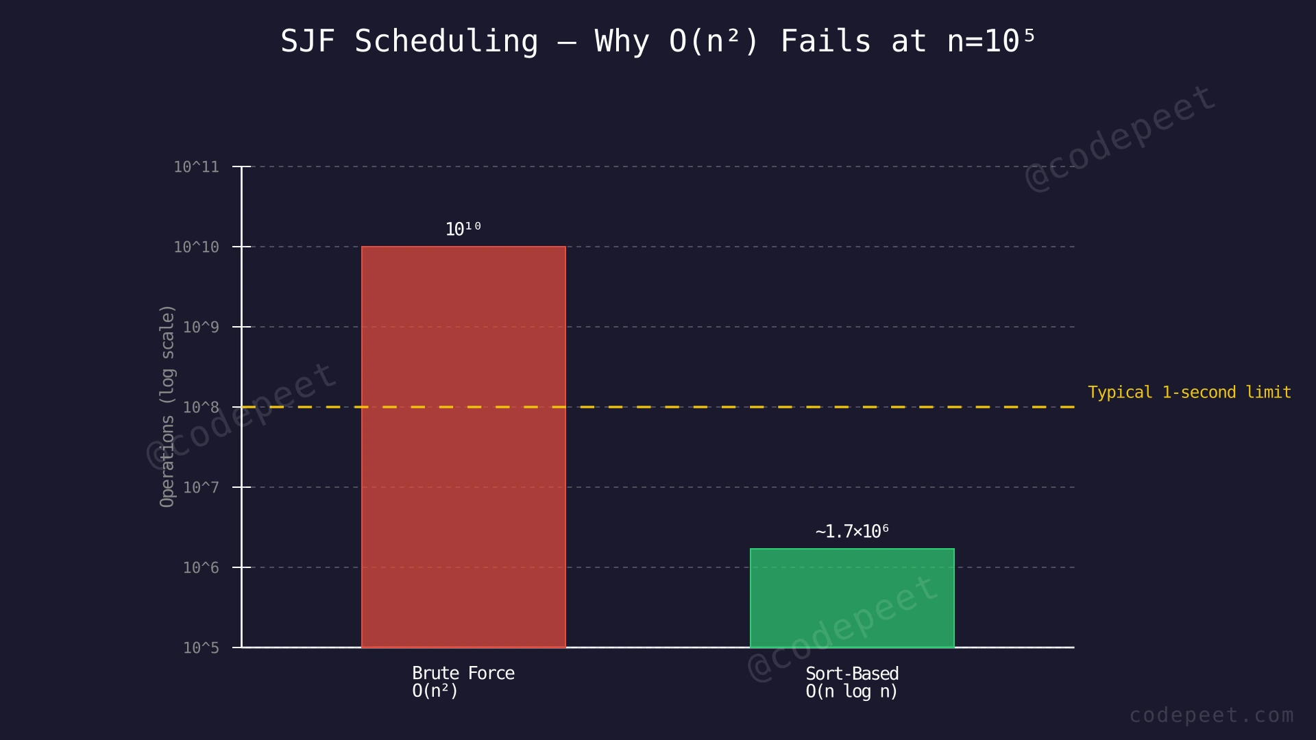
We perform n rounds of scheduling. In each round, we scan up to n processes to find the minimum burst time. This gives n × n = n² total comparisons in the worst case. For n = 10^5, that is up to 10^10 operations.
Space Complexity: O(n)
We use a boolean array done[] of size n to track which processes have already been executed. All other variables use constant space.
Why This Approach Is Not Efficient
The brute force approach performs a linear scan in every round to find the minimum burst time. With n processes, we do n rounds of scanning, and each scan touches up to n elements. This results in O(n²) total work.
For n = 10^5, that means up to 10^10 comparisons — far exceeding the typical time limit of ~10^8 operations per second. The algorithm would take roughly 100 seconds instead of the allowed 1-2 seconds.
The root inefficiency is that we are repeatedly solving the same sub-problem: finding the minimum element from an unsorted collection. Each time we find and remove the minimum, the next round starts from scratch, re-scanning elements we have already compared.
Key insight: If we sort the burst times once upfront, they are already arranged from shortest to longest — exactly the order SJF needs. Sorting costs O(n log n), and then computing waiting times is a single O(n) pass. The total O(n log n) is dramatically faster than O(n²) for large inputs.
Optimal Approach — Sort and Compute
Intuition
The SJF policy says: always execute the process with the shortest burst time next. If all processes arrive at time 0, the optimal execution order is simply the burst times arranged from smallest to largest.
Instead of repeatedly scanning for the minimum (which is what the brute force does), we can sort the burst times once and then process them in sorted order. Sorting arranges the jobs exactly as SJF would schedule them.
Once sorted, computing waiting times becomes trivial: the i-th process in the sorted order waited for all the processes before it to finish. So its waiting time is the running sum of burst times of processes 0 through i-1. This is just a prefix sum.
Think of it like a queue at a bank. If everyone lines up by how long their transaction takes (shortest first), you minimize the total waiting time for all customers. Sorting gives us this optimal line-up instantly.
Step-by-Step Explanation
Let's trace through with bt = [4, 3, 7, 1, 2]:
Step 1: Start with the unsorted burst times: [4, 3, 7, 1, 2].
Step 2: Sort the array in ascending order: [1, 2, 3, 4, 7]. This gives us the SJF execution order — shortest burst first.
Step 3: Process the first job (burst = 1). It starts immediately at time 0, so waiting time = 0. After it finishes, current time = 0 + 1 = 1.
Step 4: Process the second job (burst = 2). It waited while the first job ran, so waiting time = 1. Current time = 1 + 2 = 3.
Step 5: Process the third job (burst = 3). It waited for the first two jobs to complete, so waiting time = 3. Current time = 3 + 3 = 6.
Step 6: Process the fourth job (burst = 4). Waiting time = 6 (sum of previous bursts: 1 + 2 + 3). Current time = 6 + 4 = 10.
Step 7: Process the last job (burst = 7). Waiting time = 10 (sum of all previous: 1 + 2 + 3 + 4). Current time = 10 + 7 = 17.
Step 8: All processes complete. Total waiting time = 0 + 1 + 3 + 6 + 10 = 20. Average = 20 / 5 = 4.
Optimal — Sort Then Compute Waiting Times — After sorting burst times, we process jobs left to right, building a running sum of waiting times in the secondary row. Each job's wait equals the cumulative burst of all preceding jobs.
Algorithm
- Sort the burst time array
btin ascending order - Initialize
current_time = 0andtotal_wait = 0 - For each burst time
bt[i]in sorted order:
a. Addcurrent_timetototal_wait(this is process i's waiting time)
b. Advancecurrent_timebybt[i] - Return
total_wait / n(integer division for floor)
Code
#include <vector>
#include <algorithm>
using namespace std;

class Solution {
public:
    long long solve(vector<int>& bt) {
        int n = bt.size();
        sort(bt.begin(), bt.end());

        long long totalWait = 0;
        long long currentTime = 0;

        for (int i = 0; i < n; i++) {
            totalWait += currentTime;
            currentTime += bt[i];
        }

        return totalWait / n;
    }
};
class Solution:
def solve(self, bt):
n = len(bt)
bt.sort()
total_wait = 0
current_time = 0
for burst in bt:
total_wait += current_time
current_time += burst
return total_wait // nimport java.util.Arrays;
class Solution {
long solve(int[] bt) {
int n = bt.length;
Arrays.sort(bt);
long totalWait = 0;
long currentTime = 0;
for (int i = 0; i < n; i++) {
totalWait += currentTime;
currentTime += bt[i];
}
return totalWait / n;
}
}Complexity Analysis
Time Complexity: O(n log n)
Sorting the burst times takes O(n log n) using an efficient comparison sort (like merge sort or introsort). The subsequent loop to compute waiting times is O(n). The dominant term is the sort, giving O(n log n) overall. For n = 10^5, this is roughly 1.7 × 10^6 operations — well within time limits.
Space Complexity: O(1) auxiliary
If we sort in-place (which most standard library sorts do), we only need a constant amount of extra space for the running variables totalWait and currentTime. The sorting itself may use O(log n) stack space for recursion, but no auxiliary data structures proportional to n are needed.