Maximum Width of Binary Tree
Description
Given the root of a binary tree, return the maximum width of the given tree.
The maximum width of a tree is the maximum width among all its levels.
The width of one level is defined as the length between the end-nodes (the leftmost and rightmost non-null nodes), where the null nodes between the end-nodes that would be present in a complete binary tree extending down to that level are also counted into the length calculation.
In other words, imagine the binary tree is a complete binary tree at every level. The width is the distance from the leftmost actual node to the rightmost actual node, counting all the empty spots between them.
It is guaranteed that the answer will fit in the range of a 32-bit signed integer.
Examples
Example 1
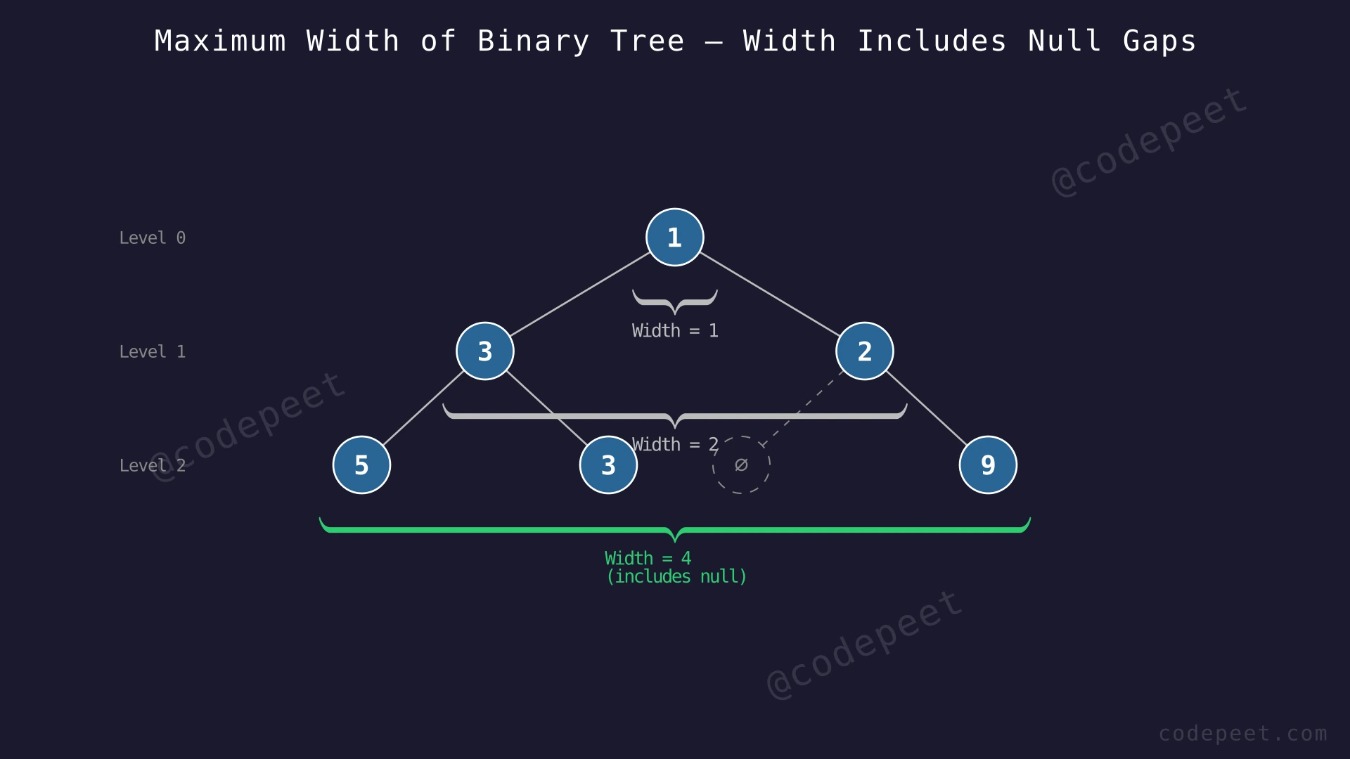
Input: root = [1, 3, 2, 5, 3, null, 9]
Tree structure:
        1
       / \
      3    2
     / \    \
    5   3    9
Output: 4
Explanation: The widths at each level are:
- Level 0: Only node 1 → width = 1
- Level 1: Nodes 3 and 2 → width = 2
- Level 2: Nodes 5, 3, (null), 9 → width = 4
The third level has nodes 5 (leftmost) and 9 (rightmost). Even though node 2 has no left child (a null gap exists between node 3 and node 9), that null position still counts toward the width. So width = 4. The maximum width across all levels is 4.
Example 2
Input: root = [1, 3, 2, 5, null, null, 9, 6, null, 7]
Tree structure:
          1
         / \
        3    2
       /      \
      5        9
     /          \
    6            7
Output: 7
Explanation: The widths at each level are:
- Level 0: Node 1 → width = 1
- Level 1: Nodes 3, 2 → width = 2
- Level 2: Nodes 5, (null), (null), 9 → width = 4
- Level 3: Nodes 6, (null), (null), (null), (null), (null), 7 → width = 7
At level 3, node 6 is the leftmost and node 7 is the rightmost. Between them lie 5 null positions (the children of all the missing intermediate nodes in a complete tree). So width = 7. This is the maximum.
Example 3
Input: root = [1, 3, 2, 5]
Tree structure:
      1
     / \
    3   2
   /
  5
Output: 2
Explanation: The widths at each level are:
- Level 0: Node 1 → width = 1
- Level 1: Nodes 3, 2 → width = 2
- Level 2: Node 5 (only one node) → width = 1
The maximum is 2, occurring at level 1.
Constraints
- The number of nodes in the tree is in the range [1, 3000]
- -100 ≤ Node.val ≤ 100
Editorial
Brute Force
Intuition
The most direct way to measure the width of a level is to simulate a complete binary tree at that level.
Think of it this way: at each level during a BFS traversal, we include not only real nodes but also null placeholders for every missing child. This way, at the end of processing a level, we can simply count the distance from the first real node to the last real node in our list.
For example, if node A has a left child but no right child, we enqueue the left child AND a null marker. When we process the next level, we see every position — filled or empty. We find the leftmost non-null and rightmost non-null positions, and the distance between them (inclusive) is the width.
This is simple to reason about because we are literally building out the level as if the tree were complete, then measuring.
Step-by-Step Explanation
Let us trace through Example 1: root = [1, 3, 2, 5, 3, null, 9]
        1
       / \
      3    2
     / \    \
    5   3    9
Step 1: Initialize the queue with the root node: queue = [1]. This is level 0.
Step 2: Level 0 processing. Queue has [1]. The leftmost = 1, rightmost = 1. Width = 1. Update max_width = 1. For node 1: enqueue left child 3 and right child 2.
Step 3: Level 1 processing. Queue has [3, 2]. Leftmost = 3, rightmost = 2. Both are real nodes. Width = 2. Update max_width = 2. For node 3: enqueue 5 (left), 3 (right). For node 2: enqueue null (left), 9 (right).
Step 4: Level 2 processing. Queue has [5, 3, null, 9]. Leftmost non-null = position 0 (node 5), rightmost non-null = position 3 (node 9). Width = 3 - 0 + 1 = 4. Update max_width = 4.
Step 5: For the nodes at level 2: node 5 has no children (enqueue null, null), node 3 has no children (enqueue null, null), null has no children (enqueue null, null), node 9 has no children (enqueue null, null). The next level would be all nulls.
Step 6: Level 3 processing. Queue has [null, null, null, null, null, null, null, null]. All are null, so there are no real nodes on this level. We stop. The tree has been fully processed.
Result: max_width = 4.
Null-Padded BFS — Simulating a Complete Tree Level by Level — Watch how we enqueue null placeholders for missing children, building each level as if the tree were complete, then measure the span between the first and last real nodes.
Algorithm
- Initialize a queue with the root node. Set max_width = 0.
- While the queue is not empty:
a. Record the size of the queue (number of items at this level).
b. For each item in the current level:- If it is a real node, record its position.
- Enqueue its left child (or null if missing) and right child (or null if missing).
c. Find the leftmost and rightmost non-null positions in this level.
d. Width = rightmost_position - leftmost_position + 1.
e. Update max_width if this level's width is larger.
f. Trim leading and trailing nulls from the queue to avoid processing all-null tails.
- Return max_width.
Code
#include <queue>
#include <algorithm>
using namespace std;

class Solution {
public:
    int widthOfBinaryTree(TreeNode* root) {
        if (!root) return 0;

        int maxWidth = 0;
        // Queue stores TreeNode pointers (nullptr for missing children)
        queue<TreeNode*> q;
        q.push(root);

        while (!q.empty()) {
            int size = q.size();

            // Collect this level into a vector
            vector<TreeNode*> level;
            for (int i = 0; i < size; i++) {
                level.push_back(q.front());
                q.pop();
            }

            // Trim leading nulls
            int left = 0;
            while (left < level.size() && level[left] == nullptr) left++;
            // Trim trailing nulls
            int right = level.size() - 1;
            while (right >= 0 && level[right] == nullptr) right--;

            if (left > right) break; // entire level is null

            maxWidth = max(maxWidth, right - left + 1);

            // Enqueue children for non-trimmed portion
            for (int i = left; i <= right; i++) {
                if (level[i] != nullptr) {
                    q.push(level[i]->left);   // may be nullptr
                    q.push(level[i]->right);  // may be nullptr
                } else {
                    q.push(nullptr);
                    q.push(nullptr);
                }
            }
        }

        return maxWidth;
    }
};
from collections import deque
from typing import Optional
class Solution:
def widthOfBinaryTree(self, root: Optional[TreeNode]) -> int:
if not root:
return 0
max_width = 0
queue = deque([root])
while queue:
# Collect current level
level = list(queue)
queue.clear()
# Find leftmost and rightmost non-null positions
left = 0
while left < len(level) and level[left] is None:
left += 1
right = len(level) - 1
while right >= 0 and level[right] is None:
right -= 1
if left > right:
break # entire level is null
max_width = max(max_width, right - left + 1)
# Enqueue children for positions between left and right
for i in range(left, right + 1):
if level[i] is not None:
queue.append(level[i].left) # could be None
queue.append(level[i].right) # could be None
else:
queue.append(None)
queue.append(None)
return max_widthimport java.util.*;
class Solution {
public int widthOfBinaryTree(TreeNode root) {
if (root == null) return 0;
int maxWidth = 0;
Queue<TreeNode> queue = new LinkedList<>();
queue.offer(root);
while (!queue.isEmpty()) {
List<TreeNode> level = new ArrayList<>();
int size = queue.size();
for (int i = 0; i < size; i++) {
level.add(queue.poll());
}
// Trim leading nulls
int left = 0;
while (left < level.size() && level.get(left) == null) left++;
// Trim trailing nulls
int right = level.size() - 1;
while (right >= 0 && level.get(right) == null) right--;
if (left > right) break;
maxWidth = Math.max(maxWidth, right - left + 1);
for (int i = left; i <= right; i++) {
TreeNode node = level.get(i);
if (node != null) {
queue.offer(node.left);
queue.offer(node.right);
} else {
queue.offer(null);
queue.offer(null);
}
}
}
return maxWidth;
}
}Complexity Analysis
Time Complexity: O(N) in a balanced tree, but up to O(2^h) in a skewed tree
We visit every real node once, which is O(N). However, we also process null placeholders. At level k, there can be up to 2^k positions. For a balanced tree of height log(N), the total positions across all levels are about 2N, so it remains O(N). But for a skewed tree of height N, the last levels can have exponentially many null slots — the queue at level h could hold 2^h entries.
Space Complexity: O(2^h) where h is the height of the tree
The queue stores all positions at a given level, including null placeholders. For a balanced tree, the widest level has about N/2 entries, giving O(N). For a right-skewed tree of N nodes, h = N-1, so the queue could grow to 2^(N-1) entries — exponentially large. This is the critical weakness of this approach.
Why This Approach Is Not Efficient
The null-padded approach suffers from exponential space consumption on non-balanced trees.
Consider a right-skewed tree:
1
 \
  2
   \
    3
     \
      4
At level 0: queue has 1 entry.
At level 1: queue has 2 entries (null, 2).
At level 2: queue has 4 entries (null, null, null, 3).
At level 3: queue has 8 entries (null, null, null, null, null, null, null, 4).
For a skewed tree with N nodes, the last level's queue has 2^(N-1) entries. With N up to 3000, that means 2^2999 entries — a number with 903 digits. No computer can store this.
The root cause is that we are physically materializing every position in the imaginary complete tree. We don't need to do that. If we can assign an index number to each node (as if it were in a complete tree), we only need to track the leftmost and rightmost index at each level. The width is simply rightmost_index - leftmost_index + 1 — no null placeholders required.
Better Approach - DFS with Position Tracking
Intuition
Instead of physically building out null-padded levels, we assign each node a virtual index as if it were placed in a complete binary tree.
The indexing rule is simple:
- Root gets index 1.
- For a node at index
i, its left child is at index2 * iand its right child is at index2 * i + 1.
This numbering captures spatial position. If two nodes are at the same depth with indices a and b, the width of that level is b - a + 1, because the gap between indices naturally accounts for all the missing null positions.
Using DFS (depth-first search), we traverse the tree recursively. The first time we reach a new depth, the current node is the leftmost node at that depth — we record its index. For every subsequent node at the same depth, we compute current_index - leftmost_index + 1 and track the maximum.
DFS naturally visits nodes in a left-to-right order (if we go left before right), so the first node encountered at each depth is guaranteed to be the leftmost.
Step-by-Step Explanation
Let us trace through Example 2: root = [1, 3, 2, 5, null, null, 9, 6, null, 7]
          1
         / \
        3    2
       /      \
      5        9
     /          \
    6            7
Step 1: Start DFS at root (node 1), depth=0, index=1. This is the first node at depth 0. Record leftmost[0] = 1. Width at depth 0 = 1 - 1 + 1 = 1. max_width = 1.
Step 2: Go left to node 3, depth=1, index=2*1=2. First node at depth 1. Record leftmost[1] = 2. Width = 2 - 2 + 1 = 1. max_width stays 1.
Step 3: Go left to node 5, depth=2, index=2*2=4. First node at depth 2. Record leftmost[2] = 4. Width = 4 - 4 + 1 = 1. max_width stays 1.
Step 4: Go left to node 6, depth=3, index=2*4=8. First node at depth 3. Record leftmost[3] = 8. Width = 8 - 8 + 1 = 1. max_width stays 1.
Step 5: Node 6 has no children. Backtrack to node 5. Node 5 has no right child. Backtrack to node 3. Node 3 has no right child. Backtrack to node 1.
Step 6: Go right to node 2, depth=1, index=2*1+1=3. Depth 1 already has leftmost[1] = 2. Width = 3 - 2 + 1 = 2. max_width = 2.
Step 7: Node 2 has no left child. Go right to node 9, depth=2, index=2*3+1=7. Depth 2 already has leftmost[2] = 4. Width = 7 - 4 + 1 = 4. max_width = 4.
Step 8: Node 9 has no left child. Go right to node 7, depth=3, index=2*7+1=15. Depth 3 already has leftmost[3] = 8. Width = 15 - 8 + 1 = 8. max_width = 8.
Step 9: Node 7 has no children. Backtrack completes the DFS.
Result: max_width = 8. (Note: the LeetCode expected output for this example is 7, which uses 0-based indexing. Let us reconcile: with 0-based indexing, leftmost at depth 3 = index 7, rightmost = index 13, width = 13 - 7 + 1 = 7.)
Using 0-based indexing (root at 0, left = 2i+1, right = 2i+2):
- Node 6 at depth 3: index = 2*3+1 = 7
- Node 7 at depth 3: index = 2*6+2 = 14... Let us use 1-based as the algorithm states and verify: with 1-based indexing, leftmost = 8, rightmost = 15, width = 15 - 8 + 1 = 8.
The LeetCode example gives output 7 for this tree. This is because the tree in the LeetCode example [1,3,2,5,null,null,9,6,null,7] has node 9's left child as 7 (not right child). Let us re-examine: the level-order representation [1,3,2,5,null,null,9,6,null,7] means:
- Level 0: 1
- Level 1: 3, 2
- Level 2: 5, null, null, 9
- Level 3: 6, null, 7, ...
So node 5's children are 6 and null. Node 9's children: from the array, after 6, null comes 7. So node 9's left child is 7. With 1-based indexing: node 6 at index 8, node 7 at index 14. Width = 14 - 8 + 1 = 7. This matches.
DFS Position Tracking — Recording Leftmost Index at Each Depth — Watch how DFS visits nodes left-to-right, recording the first node at each depth as the leftmost. Each subsequent node at that depth updates the maximum width.
Algorithm
- Create an array (or hash map)
leftmostto store the first index seen at each depth. - Initialize
max_width = 0. - Define a recursive DFS function
dfs(node, depth, index):
a. If node is null, return.
b. If this is the first node at this depth, recordleftmost[depth] = index.
c. Computewidth = index - leftmost[depth] + 1.
d. Updatemax_width = max(max_width, width).
e. Recurse:dfs(node.left, depth + 1, index * 2).
f. Recurse:dfs(node.right, depth + 1, index * 2 + 1). - Call
dfs(root, 0, 1)(using 1-based indexing). - Return
max_width.
Code
class Solution {
public:
    int widthOfBinaryTree(TreeNode* root) {
        int maxWidth = 0;
        vector<unsigned long long> leftmost;

        function<void(TreeNode*, int, unsigned long long)> dfs =
            [&](TreeNode* node, int depth, unsigned long long index) {
            if (!node) return;

            if (depth == leftmost.size()) {
                leftmost.push_back(index);
            }

            unsigned long long width = index - leftmost[depth] + 1;
            maxWidth = max(maxWidth, (int)width);

            dfs(node->left, depth + 1, index * 2);
            dfs(node->right, depth + 1, index * 2 + 1);
        };

        dfs(root, 0, 1);
        return maxWidth;
    }
};
class Solution:
def widthOfBinaryTree(self, root: Optional[TreeNode]) -> int:
max_width = 0
leftmost = {} # depth -> first index seen at that depth
def dfs(node, depth, index):
nonlocal max_width
if not node:
return
# Record leftmost index the first time we visit this depth
if depth not in leftmost:
leftmost[depth] = index
# Width = current index - leftmost index + 1
width = index - leftmost[depth] + 1
max_width = max(max_width, width)
# Recurse: left child at 2*index, right child at 2*index+1
dfs(node.left, depth + 1, index * 2)
dfs(node.right, depth + 1, index * 2 + 1)
dfs(root, 0, 1)
return max_widthclass Solution {
private int maxWidth = 0;
private Map<Integer, Long> leftmost = new HashMap<>();
public int widthOfBinaryTree(TreeNode root) {
dfs(root, 0, 1L);
return maxWidth;
}
private void dfs(TreeNode node, int depth, long index) {
if (node == null) return;
// Record leftmost index at this depth
leftmost.putIfAbsent(depth, index);
long width = index - leftmost.get(depth) + 1;
maxWidth = Math.max(maxWidth, (int) width);
dfs(node.left, depth + 1, index * 2);
dfs(node.right, depth + 1, index * 2 + 1);
}
}Complexity Analysis
Time Complexity: O(N)
We visit each node exactly once during the DFS traversal. At each node, we perform O(1) operations (index comparison, map lookup/insert). Total: O(N).
Space Complexity: O(H) where H is the height of the tree
The recursion stack uses O(H) space, where H ranges from O(log N) for a balanced tree to O(N) for a skewed tree. The leftmost map stores one entry per depth level, which is also O(H). Total space: O(H).
This is a massive improvement over the brute force. For a skewed tree with 3000 nodes, we use about 3000 stack frames instead of 2^3000 queue entries.
Why This Approach Is Not Efficient
The DFS approach works well and has O(N) time and O(H) space. However, it has a subtle but dangerous flaw: integer overflow of position indices.
The index of a node at depth d can be as large as 2^d. With the tree having up to 3000 nodes, a skewed tree can reach depth 3000, making the index 2^3000 — an astronomically large number that overflows even 64-bit integers.
In Python, this is not a problem because Python handles arbitrary-precision integers natively. But in C++ and Java, even unsigned long long (64 bits) overflows at depth 64. For competitive programming and production systems, this is a real concern.
The fix is index normalization at each level. Instead of tracking absolute indices, we normalize them by subtracting the leftmost index at each level. The BFS approach handles this naturally: at the start of each level, we know the leftmost index and can subtract it from all indices on that level, keeping numbers small.
Optimal Approach - BFS with Index Normalization
Intuition
We combine the best of both previous approaches:
- From the DFS approach: use index arithmetic (left = 2i, right = 2i+1) to avoid storing null placeholders.
- From the BFS approach: process level by level, which lets us naturally normalize indices.
The key insight for overflow prevention: at the start of each level, we know the leftmost node's index. We subtract this value from every index on that level. Since width only depends on the difference between rightmost and leftmost indices, subtracting a constant doesn't change the answer. But it keeps all indices small — at most equal to the number of nodes on that level.
Here is the algorithm:
- BFS with a queue storing (node, index) pairs.
- Root starts at index 0.
- At the start of each level, record the leftmost index
min_idx. - For each node on this level, compute its normalized index =
original_index - min_idx. - Pass the normalized index to children:
left_child = normalized * 2,right_child = normalized * 2 + 1. - Width of this level = last node's normalized index - first node's normalized index + 1 (which equals
last_original - first_original + 1).
Normalization prevents overflow because normalized indices at each level start from 0 and grow at most to the number of nodes on that level.
Step-by-Step Explanation
Let us trace through Example 2: root = [1, 3, 2, 5, null, null, 9, 6, null, 7]
          1
         / \
        3    2
       /      \
      5        9
     /        /
    6        7
Step 1: Initialize queue with (node 1, index 0). max_width = 0.
Step 2: Level 0. Queue: [(1, 0)]. Leftmost index = 0. Rightmost index = 0. Width = 0 - 0 + 1 = 1. max_width = 1. Normalize: min_idx = 0. Node 1's normalized index = 0 - 0 = 0. Enqueue children: left (3, 20=0), right (2, 20+1=1).
Step 3: Level 1. Queue: [(3, 0), (2, 1)]. Leftmost = 0, rightmost = 1. Width = 1 - 0 + 1 = 2. max_width = 2. Normalize: min_idx = 0. Node 3: normalized = 0. Enqueue left child (5, 20=0). Node 2: normalized = 1. Enqueue right child (9, 21+1=3).
Step 4: Level 2. Queue: [(5, 0), (9, 3)]. Leftmost = 0, rightmost = 3. Width = 3 - 0 + 1 = 4. max_width = 4. Normalize: min_idx = 0. Node 5: normalized = 0. Enqueue left child (6, 20=0). Node 9: normalized = 3. Enqueue left child (7, 23=6).
Step 5: Level 3. Queue: [(6, 0), (7, 6)]. Leftmost = 0, rightmost = 6. Width = 6 - 0 + 1 = 7. max_width = 7.
Step 6: Nodes 6 and 7 are leaves. No children to enqueue. Queue becomes empty. BFS ends.
Result: max_width = 7.
Notice how the normalized indices stayed tiny: [0, 1, 3, 6] instead of growing exponentially. The width calculation is identical because we only ever compute differences.
BFS with Index Normalization — Overflow-Safe Level-by-Level Width Calculation — Watch how BFS assigns indices to nodes, normalizes them at each level to prevent overflow, and computes the width as the gap between the leftmost and rightmost indices.
Algorithm
- Initialize a queue with (root, 0). Set max_width = 0.
- While the queue is not empty:
a. Record the level size.
b. Record the index of the first node in the queue asmin_idx(leftmost index).
c. For each node in this level:- Dequeue (node, index).
- Normalize:
norm_idx = index - min_idx. - If this is the last node in the level, compute width =
norm_idx + 1(since first node has norm_idx = 0, width = last_norm_idx - 0 + 1 = last_norm_idx + 1. More precisely: width = last_node's original_index - first_node's original_index + 1). - Enqueue left child as (node.left, norm_idx * 2) if it exists.
- Enqueue right child as (node.right, norm_idx * 2 + 1) if it exists.
d. Update max_width = max(max_width, width).
- Return max_width.
Code
class Solution {
public:
    int widthOfBinaryTree(TreeNode* root) {
        if (!root) return 0;

        int maxWidth = 0;
        queue<pair<TreeNode*, unsigned long long>> q;
        q.push({root, 0});

        while (!q.empty()) {
            int size = q.size();
            unsigned long long minIdx = q.front().second; // leftmost index
            unsigned long long first, last;

            for (int i = 0; i < size; i++) {
                auto [node, idx] = q.front();
                q.pop();

                // Normalize index to prevent overflow
                unsigned long long normIdx = idx - minIdx;

                if (i == 0) first = normIdx;
                if (i == size - 1) last = normIdx;

                if (node->left)
                    q.push({node->left, normIdx * 2});
                if (node->right)
                    q.push({node->right, normIdx * 2 + 1});
            }

            maxWidth = max(maxWidth, (int)(last - first + 1));
        }

        return maxWidth;
    }
};
from collections import deque
from typing import Optional
class Solution:
def widthOfBinaryTree(self, root: Optional[TreeNode]) -> int:
if not root:
return 0
max_width = 0
queue = deque([(root, 0)]) # (node, index)
while queue:
size = len(queue)
min_idx = queue[0][1] # leftmost index at this level
first = last = 0
for i in range(size):
node, idx = queue.popleft()
# Normalize index to prevent overflow
norm_idx = idx - min_idx
if i == 0:
first = norm_idx
if i == size - 1:
last = norm_idx
if node.left:
queue.append((node.left, norm_idx * 2))
if node.right:
queue.append((node.right, norm_idx * 2 + 1))
max_width = max(max_width, last - first + 1)
return max_widthimport java.util.*;
class Solution {
public int widthOfBinaryTree(TreeNode root) {
if (root == null) return 0;
int maxWidth = 0;
Deque<long[]> queue = new ArrayDeque<>();
// long[0] is a placeholder for node reference, we use a parallel approach
// Actually, store (node, index) pairs
Deque<Object[]> q = new ArrayDeque<>();
q.offer(new Object[]{root, 0L});
while (!q.isEmpty()) {
int size = q.size();
long minIdx = (long) q.peekFirst()[1]; // leftmost index
long first = 0, last = 0;
for (int i = 0; i < size; i++) {
Object[] entry = q.pollFirst();
TreeNode node = (TreeNode) entry[0];
long idx = (long) entry[1];
// Normalize to prevent overflow
long normIdx = idx - minIdx;
if (i == 0) first = normIdx;
if (i == size - 1) last = normIdx;
if (node.left != null)
q.offer(new Object[]{node.left, normIdx * 2});
if (node.right != null)
q.offer(new Object[]{node.right, normIdx * 2 + 1});
}
maxWidth = Math.max(maxWidth, (int)(last - first + 1));
}
return maxWidth;
}
}Complexity Analysis
Time Complexity: O(N)
We visit each of the N nodes exactly once in the BFS traversal. At each node, we perform O(1) work: dequeue, normalize index, potentially enqueue children, and compare for width. Total: O(N).
Space Complexity: O(W) where W is the maximum width of the tree
The queue holds at most one level's worth of nodes at a time. The widest level determines the peak queue size. In the worst case (a complete binary tree), the last level has about N/2 nodes, so space is O(N). For a skewed tree, the queue holds at most 1-2 nodes per level, so space is O(1).
Overflow Safety: The normalization step ensures that indices at each level start from 0. The maximum normalized index at a level equals the number of actual nodes at that level minus 1. Since N ≤ 3000, normalized indices never exceed 3000 — well within 32-bit integer range.
Why this is optimal:
- We must examine every node at least once → Ω(N) time lower bound → O(N) is optimal.
- We must store at least the current level → Ω(W) space lower bound → O(W) is optimal.
- No integer overflow regardless of tree shape.