Binary Tree Representation
Description
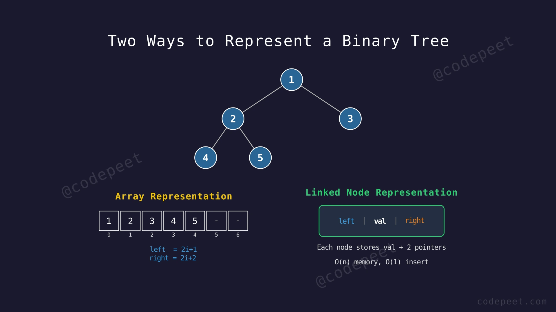
A binary tree is a hierarchical data structure where each node has at most two children, referred to as the left child and the right child. The topmost node is called the root, and nodes with no children are called leaves.
The challenge is: how do we store a binary tree in computer memory? There are two primary approaches:
- Array (Sequential) Representation — Store nodes in a flat array using index arithmetic to navigate parent-child relationships.
- Linked Node (Pointer) Representation — Each node is an object containing data and pointers (references) to its left and right children.
Given a binary tree with N nodes, implement both representations and support these operations:
- insert(value) — Insert a new node in level-order (left to right, top to bottom).
- getLeftChild(node) — Return the left child of the given node.
- getRightChild(node) — Return the right child of the given node.
- getParent(node) — Return the parent of the given node.
- levelOrderTraversal() — Print all nodes level by level.
Understand the trade-offs between the two representations in terms of memory usage, flexibility, and access speed.
Examples
Example 1
Input:
Insert values in order: 1, 2, 3, 4, 5, 6
Tree structure formed (level-order insertion):
       1
      / \
     2   3
    / \  /
   4  5  6
Array representation: [1, 2, 3, 4, 5, 6]
Queries:
- getLeftChild(index 0) → index 1, value 2
- getRightChild(index 0) → index 2, value 3
- getParent(index 4) → index 1, value 2
- levelOrderTraversal() → [1, 2, 3, 4, 5, 6]
Explanation: When inserting in level-order, each level fills left to right before moving to the next level. Node 1 is the root (index 0). Its left child is at index 2×0+1=1 (value 2) and right child at 2×0+2=2 (value 3). Node 5 at index 4 has parent at (4-1)/2=1 (value 2).
Example 2
Input (sparse/skewed tree):
Tree:
  1
   \
    3
     \
      7
Array representation: [1, null, 3, null, null, null, 7]
The array needs 7 slots even though only 3 nodes exist. Indices 1, 3, 4, 5 are wasted (null).
Linked representation: Only 3 node objects created — no wasted memory.
Explanation: For a right-skewed tree of height h, the array needs 2^(h+1) - 1 slots but only h+1 are filled. This tree has height 2, requiring 7 array slots for 3 nodes — over 57% waste. With linked nodes, we allocate memory only for existing nodes.
Example 3
Input:
Insert value: 42
Tree structure: A single root node.
42
Array representation: [42]
Linked representation: One node with data=42, left=null, right=null.
Explanation: The simplest binary tree has one node. Both representations are equivalent here — one array cell or one node object.
Constraints
- 1 ≤ N ≤ 10^5 (number of nodes)
- Node values are integers in the range [-10^9, 10^9]
- The binary tree is a general binary tree (not necessarily complete or balanced)
- For array representation, the maximum height h determines array size: up to 2^(h+1) - 1 slots
- Each node has at most 2 children (left and right)
Editorial
Brute Force
Intuition
The simplest way to represent a binary tree is to lay it flat inside an array, using index arithmetic to encode parent-child relationships.
Think of a spreadsheet with numbered rows. You place the root in row 0. For any node in row i, its left child goes in row 2i + 1 and its right child in row 2i + 2. To find a node's parent, you compute (i - 1) / 2 (integer division). No pointers, no references — just simple math.
This approach works beautifully for complete binary trees where every level is fully filled (except possibly the last). The array has no gaps, and every index maps to a real node.
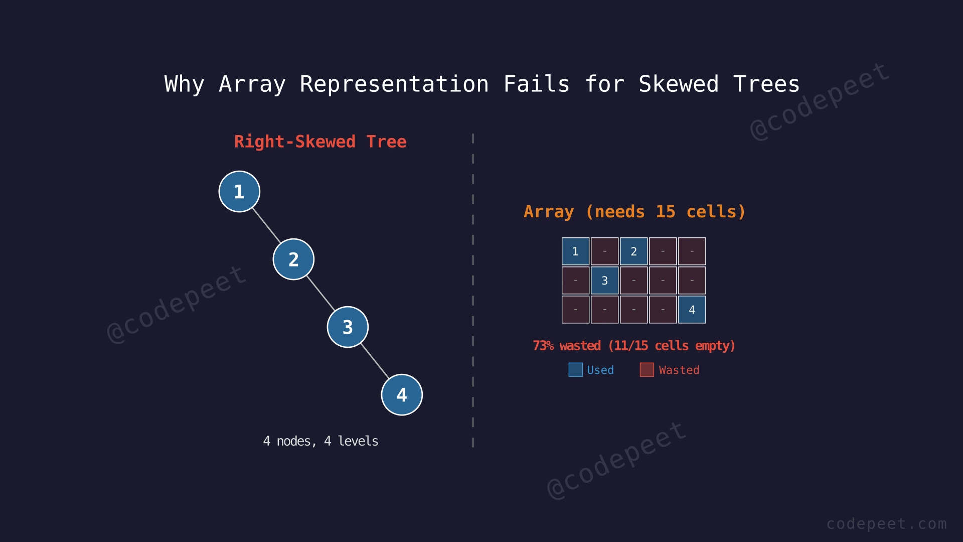
However, for sparse or skewed trees, the story changes. If a node at depth d only has a right child, you must still reserve the left child's array index (it stays null). A fully right-skewed tree of n nodes requires an array of size 2^n - 1 — exponentially more space than needed.
Step-by-Step Explanation
Let us build the tree from Example 1 using an array and then perform queries.
Tree to build:
       1
      / \
     2   3
    / \  /
   4  5  6
Step 1: Create an array of capacity 7 (enough for 3 levels). Initialize all slots to null.
Step 2: Insert root value 1 at index 0. The root always occupies index 0.
Step 3: Insert 2 as left child of root (index 0). Left child index = 2×0 + 1 = 1. Place 2 at index 1.
Step 4: Insert 3 as right child of root (index 0). Right child index = 2×0 + 2 = 2. Place 3 at index 2.
Step 5: Insert 4 as left child of node at index 1. Left child index = 2×1 + 1 = 3. Place 4 at index 3.
Step 6: Insert 5 as right child of node at index 1. Right child index = 2×1 + 2 = 4. Place 5 at index 4.
Step 7: Insert 6 as left child of node at index 2. Left child index = 2×2 + 1 = 5. Place 6 at index 5.
Step 8: Array is now [1, 2, 3, 4, 5, 6, null]. All 6 nodes stored.
Step 9: Query — left child of root? Index = 2×0 + 1 = 1. Array[1] = 2. Answer: 2. Instant O(1) lookup using pure arithmetic.
Step 10: Query — parent of node at index 4 (value 5)? Parent index = (4-1)/2 = 1. Array[1] = 2. Answer: 2 is the parent of 5.
Array Representation — Building a Binary Tree in a Flat Array — Watch how nodes are placed at computed array indices using the formulas: left child = 2i+1, right child = 2i+2.
Algorithm
Initialization:
- Determine the maximum height
hof the tree. - Create an array of size
2^(h+1) - 1, initialized to a sentinel value (e.g., null or -1).
Insert (level-order):
- Find the first empty slot by scanning the array in order, or track the next insertion index.
- Place the value at that index.
getLeftChild(i):
- Compute index =
2 * i + 1. - If index is within bounds and not null, return array[index].
getRightChild(i):
- Compute index =
2 * i + 2. - If index is within bounds and not null, return array[index].
getParent(i):
- If i == 0, return null (root has no parent).
- Compute index =
(i - 1) / 2. - Return array[index].
levelOrderTraversal:
- Iterate through the array from index 0 to end.
- Print all non-null values.
Code
#include <vector>
#include <iostream>
#include <queue>
using namespace std;

class BinaryTreeArray {
    vector<int> tree;
    vector<bool> occupied;
    int capacity;

public:
    BinaryTreeArray(int maxNodes) {
        capacity = maxNodes;
        tree.resize(capacity, 0);
        occupied.resize(capacity, false);
    }

    void setRoot(int val) {
        tree[0] = val;
        occupied[0] = true;
    }

    void setLeft(int parentIdx, int val) {
        int idx = 2 * parentIdx + 1;
        if (idx < capacity && occupied[parentIdx]) {
            tree[idx] = val;
            occupied[idx] = true;
        }
    }

    void setRight(int parentIdx, int val) {
        int idx = 2 * parentIdx + 2;
        if (idx < capacity && occupied[parentIdx]) {
            tree[idx] = val;
            occupied[idx] = true;
        }
    }

    int getLeftChild(int idx) {
        int left = 2 * idx + 1;
        if (left < capacity && occupied[left])
            return tree[left];
        return -1; // no left child
    }

    int getRightChild(int idx) {
        int right = 2 * idx + 2;
        if (right < capacity && occupied[right])
            return tree[right];
        return -1; // no right child
    }

    int getParent(int idx) {
        if (idx == 0) return -1; // root
        int parent = (idx - 1) / 2;
        return tree[parent];
    }

    void levelOrder() {
        for (int i = 0; i < capacity; i++) {
            if (occupied[i])
                cout << tree[i] << " ";
        }
        cout << endl;
    }
};
class BinaryTreeArray:
def __init__(self, max_nodes):
self.capacity = max_nodes
self.tree = [None] * max_nodes
def set_root(self, val):
self.tree[0] = val
def set_left(self, parent_idx, val):
idx = 2 * parent_idx + 1
if idx < self.capacity and self.tree[parent_idx] is not None:
self.tree[idx] = val
def set_right(self, parent_idx, val):
idx = 2 * parent_idx + 2
if idx < self.capacity and self.tree[parent_idx] is not None:
self.tree[idx] = val
def get_left_child(self, idx):
left = 2 * idx + 1
if left < self.capacity and self.tree[left] is not None:
return self.tree[left]
return None
def get_right_child(self, idx):
right = 2 * idx + 2
if right < self.capacity and self.tree[right] is not None:
return self.tree[right]
return None
def get_parent(self, idx):
if idx == 0:
return None # root has no parent
parent = (idx - 1) // 2
return self.tree[parent]
def level_order(self):
result = []
for i in range(self.capacity):
if self.tree[i] is not None:
result.append(self.tree[i])
return resultimport java.util.*;
class BinaryTreeArray {
Integer[] tree;
int capacity;
BinaryTreeArray(int maxNodes) {
capacity = maxNodes;
tree = new Integer[capacity];
}
void setRoot(int val) {
tree[0] = val;
}
void setLeft(int parentIdx, int val) {
int idx = 2 * parentIdx + 1;
if (idx < capacity && tree[parentIdx] != null) {
tree[idx] = val;
}
}
void setRight(int parentIdx, int val) {
int idx = 2 * parentIdx + 2;
if (idx < capacity && tree[parentIdx] != null) {
tree[idx] = val;
}
}
Integer getLeftChild(int idx) {
int left = 2 * idx + 1;
if (left < capacity && tree[left] != null)
return tree[left];
return null;
}
Integer getRightChild(int idx) {
int right = 2 * idx + 2;
if (right < capacity && tree[right] != null)
return tree[right];
return null;
}
Integer getParent(int idx) {
if (idx == 0) return null;
int parent = (idx - 1) / 2;
return tree[parent];
}
List<Integer> levelOrder() {
List<Integer> result = new ArrayList<>();
for (int i = 0; i < capacity; i++) {
if (tree[i] != null)
result.add(tree[i]);
}
return result;
}
}Complexity Analysis
getLeftChild / getRightChild / getParent: O(1)
Each operation is a single arithmetic computation plus one array access. This is the major strength of array representation — navigation is pure index math, no pointer chasing.
levelOrderTraversal: O(capacity)
We scan the entire array. For a complete tree, capacity ≈ N, so it is O(N). For a sparse tree, capacity can be much larger than N.
Space Complexity: O(2^(h+1)) where h is the tree height
This is the critical weakness. The array must be large enough to hold a node at any position, even if most positions are empty. For a complete tree of N nodes, h = log₂(N), so space = O(N) — efficient. But for a skewed tree of N nodes, h = N-1, so space = O(2^N) — exponentially wasteful.
Example of waste: A right-skewed tree with 20 nodes has height 19. The array needs 2^20 - 1 = 1,048,575 slots for just 20 nodes. That is over 99.99% waste.
Why This Approach Is Not Efficient
The array representation has two fundamental problems:
1. Exponential Space Waste for Non-Complete Trees
The array size must accommodate the deepest possible node. For a skewed tree (essentially a linked list), the last node sits at index 2^h - 1 where h is the height. With N nodes in a skewed tree, h = N-1, so the array needs 2^N - 1 slots for just N nodes.
With N up to 10^5, a skewed tree would need an array of size 2^(10^5), which is astronomically larger than any available memory. Even a moderately unbalanced tree with height 30 requires over a billion slots.
2. No Dynamic Resizing
The array size must be fixed upfront. If we guess too small, we cannot insert deeper nodes. If we guess too large, we waste memory. There is no good middle ground for arbitrary tree shapes.
3. Insertion and Deletion are Awkward
Deleting a node from the middle of the tree may leave gaps. Restructuring (e.g., after deletions) requires shifting large portions of the array.
The core insight: Instead of reserving space for every possible position, we should allocate memory only for nodes that actually exist. Each node stores its own pointers (left, right), so the tree shape is encoded in the connections themselves — not in index arithmetic. This is the linked node representation.
Optimal Approach - Linked Node Representation
Intuition
Instead of fitting a tree into a rigid array, we let the tree define its own shape. Each node is an independent object that carries three pieces of information:
- Data — the value stored in the node.
- Left pointer — a reference to the left child (or null if no left child).
- Right pointer — a reference to the right child (or null if no right child).
Think of it like a family tree on paper. Instead of reserving a grid of slots, each person's card simply lists who their children are. If someone has no children, their card says 'none'. You only create cards for people who actually exist.
To insert a new node, we create a fresh object and update one pointer in the parent. To delete a node, we redirect pointers. No array resizing, no index arithmetic, no wasted slots for absent nodes.
Memory usage scales with the actual number of nodes: N nodes require exactly N objects, each with a fixed overhead for the two pointers. For a skewed tree of 20 nodes, we use 20 objects — not a million array slots.
The only trade-off is that finding the parent requires either an extra parent pointer per node or a search. We solve this by optionally storing a parent reference in each node — a small cost for O(1) parent access.
Step-by-Step Explanation
Let us build the same tree using linked nodes and then perform queries.
Tree to build:
       1
      / \
     2   3
    / \  /
   4  5  6
Step 1: Create root node: Node(1) with left=null, right=null.
Step 2: Create Node(2). Set root.left = Node(2). The left pointer of node 1 now references node 2.
Step 3: Create Node(3). Set root.right = Node(3). The right pointer of node 1 now references node 3.
Step 4: Create Node(4). Set Node(2).left = Node(4). Node 2's left pointer connects to node 4.
Step 5: Create Node(5). Set Node(2).right = Node(5). Node 2's right pointer connects to node 5.
Step 6: Create Node(6). Set Node(3).left = Node(6). Node 3's left pointer connects to node 6. Node 3 has no right child — its right pointer simply stays null. Zero wasted memory.
Step 7: Construction complete. We allocated exactly 6 node objects — one per tree node. No slots wasted regardless of tree shape.
Step 8: Query — left child of root? Follow root.left pointer → arrives at Node(2), value = 2. One pointer dereference.
Step 9: Query — right child of Node(2)? Follow Node(2).right pointer → arrives at Node(5), value = 5. Again one pointer hop.
Step 10: Query — parent of Node(5)? If we store parent pointers, follow Node(5).parent → Node(2), value = 2. Without parent pointers, we would search from root, taking O(h) time.
Linked Node Representation — Building the Tree Node by Node — Watch as each node is created and connected via pointers, forming the tree structure dynamically with zero wasted space.
Algorithm
Node Definition:
- Each node stores:
data,leftpointer,rightpointer. - Optionally:
parentpointer for O(1) parent access.
Insert (level-order using BFS):
- If tree is empty, create root with the given value.
- Otherwise, use a queue. Start with root in the queue.
- Dequeue a node:
- If its left child is null, insert the new node as left child. Done.
- If its right child is null, insert the new node as right child. Done.
- Otherwise, enqueue both children.
- Repeat until insertion is complete.
getLeftChild(node):
- Return node.left (may be null).
getRightChild(node):
- Return node.right (may be null).
getParent(node):
- If parent pointer is stored: return node.parent.
- Otherwise: search from root using DFS/BFS to find the node's parent.
levelOrderTraversal:
- Use a queue. Enqueue root.
- While queue is not empty: dequeue, print value, enqueue non-null children.
Code
#include <iostream>
#include <queue>
using namespace std;

class Node {
public:
    int data;
    Node* left;
    Node* right;

    Node(int val) {
        data = val;
        left = nullptr;
        right = nullptr;
    }
};

class BinaryTreeLinked {
    Node* root;

public:
    BinaryTreeLinked() : root(nullptr) {}

    void insert(int val) {
        Node* newNode = new Node(val);
        if (root == nullptr) {
            root = newNode;
            return;
        }
        // Level-order insertion using BFS
        queue<Node*> q;
        q.push(root);
        while (!q.empty()) {
            Node* curr = q.front();
            q.pop();
            if (curr->left == nullptr) {
                curr->left = newNode;
                return;
            }
            q.push(curr->left);
            if (curr->right == nullptr) {
                curr->right = newNode;
                return;
            }
            q.push(curr->right);
        }
    }

    Node* getRoot() {
        return root;
    }

    Node* getLeftChild(Node* node) {
        return (node != nullptr) ? node->left : nullptr;
    }

    Node* getRightChild(Node* node) {
        return (node != nullptr) ? node->right : nullptr;
    }

    void levelOrder() {
        if (root == nullptr) return;
        queue<Node*> q;
        q.push(root);
        while (!q.empty()) {
            Node* curr = q.front();
            q.pop();
            cout << curr->data << " ";
            if (curr->left) q.push(curr->left);
            if (curr->right) q.push(curr->right);
        }
        cout << endl;
    }
};
from collections import deque
class Node:
def __init__(self, val):
self.data = val
self.left = None
self.right = None
class BinaryTreeLinked:
def __init__(self):
self.root = None
def insert(self, val):
new_node = Node(val)
if self.root is None:
self.root = new_node
return
# Level-order insertion using BFS
queue = deque([self.root])
while queue:
curr = queue.popleft()
if curr.left is None:
curr.left = new_node
return
queue.append(curr.left)
if curr.right is None:
curr.right = new_node
return
queue.append(curr.right)
def get_root(self):
return self.root
def get_left_child(self, node):
return node.left if node else None
def get_right_child(self, node):
return node.right if node else None
def level_order(self):
if not self.root:
return []
result = []
queue = deque([self.root])
while queue:
curr = queue.popleft()
result.append(curr.data)
if curr.left:
queue.append(curr.left)
if curr.right:
queue.append(curr.right)
return resultimport java.util.*;
class Node {
int data;
Node left, right;
Node(int val) {
data = val;
left = null;
right = null;
}
}
class BinaryTreeLinked {
Node root;
BinaryTreeLinked() {
root = null;
}
void insert(int val) {
Node newNode = new Node(val);
if (root == null) {
root = newNode;
return;
}
// Level-order insertion using BFS
Queue<Node> q = new LinkedList<>();
q.add(root);
while (!q.isEmpty()) {
Node curr = q.poll();
if (curr.left == null) {
curr.left = newNode;
return;
}
q.add(curr.left);
if (curr.right == null) {
curr.right = newNode;
return;
}
q.add(curr.right);
}
}
Node getRoot() {
return root;
}
Node getLeftChild(Node node) {
return (node != null) ? node.left : null;
}
Node getRightChild(Node node) {
return (node != null) ? node.right : null;
}
List<Integer> levelOrder() {
List<Integer> result = new ArrayList<>();
if (root == null) return result;
Queue<Node> q = new LinkedList<>();
q.add(root);
while (!q.isEmpty()) {
Node curr = q.poll();
result.add(curr.data);
if (curr.left != null) q.add(curr.left);
if (curr.right != null) q.add(curr.right);
}
return result;
}
}Complexity Analysis
Insert (level-order BFS): O(N)
In the worst case, we traverse all existing nodes via BFS before finding an empty child slot. This takes O(N) where N is the current number of nodes.
getLeftChild / getRightChild: O(1)
A single pointer dereference. This matches the array representation's O(1) index access.
getParent (with parent pointer): O(1)
If each node stores a reference to its parent, looking up the parent is one pointer dereference.
getParent (without parent pointer): O(N)
Without a stored parent pointer, we must search from the root using BFS or DFS, which takes O(N) in the worst case.
levelOrderTraversal: O(N)
We visit each of the N nodes exactly once using BFS.
Space Complexity: O(N)
We store exactly N node objects. Each node has a fixed-size overhead (data + 2 pointers). The total memory is proportional to N regardless of tree shape — whether the tree is perfectly balanced or completely skewed.
Comparison with Array Representation:
| Aspect | Array | Linked Nodes |
|---|---|---|
| Space (complete tree) | O(N) | O(N) |
| Space (skewed tree) | O(2^N) | O(N) |
| Left/Right child | O(1) math | O(1) pointer |
| Parent access | O(1) math | O(1) with parent pointer |
| Insert at leaf | O(1) | O(N) BFS |
| Dynamic resize | Not possible | Naturally dynamic |
| Best suited for | Complete / nearly complete trees | Any tree shape |
The linked representation is the standard choice for binary trees in practice because real-world trees are rarely perfectly complete. Its O(N) space guarantee for any shape makes it universally safe, while the array representation's O(2^N) worst case makes it unsuitable for general binary trees.