Graph Types & Terminology
Description
A graph is a non-linear data structure made up of vertices (also called nodes) and edges (also called links or arcs) that represent relationships between objects.
Formally, a graph G is defined as an ordered pair G = (V, E), where:
- V is the set of vertices (the objects)
- E is the set of edges (the connections between objects)
Unlike arrays or linked lists that follow a sequential order, and unlike trees that follow a strict hierarchy, graphs have no such constraints. Any vertex can connect to any other vertex in any pattern — including back to itself.
Key Terminology:
- Vertex (Node): A fundamental unit of the graph representing an entity
- Edge (Arc/Link): A connection between two vertices
- Degree: The number of edges connected to a vertex. In directed graphs, we distinguish in-degree (edges coming in) and out-degree (edges going out)
- Path: A sequence of vertices where each adjacent pair is connected by an edge
- Cycle: A path that starts and ends at the same vertex
- Adjacent: Two vertices are adjacent if there is an edge connecting them
- Connected Graph: A graph where there is a path between every pair of vertices
- Disconnected Graph: A graph where some vertices cannot be reached from others
- Connected Component: A maximal set of vertices such that every pair has a path between them
Graph Types:
- Undirected Graph: Edges have no direction — if vertex A connects to B, then B also connects to A
- Directed Graph (Digraph): Each edge has a direction — an edge from A to B does not imply an edge from B to A
- Weighted Graph: Each edge carries a numerical value (weight) representing cost, distance, or capacity
- Unweighted Graph: All edges are treated equally with no associated weight
- Cyclic Graph: Contains at least one cycle
- Acyclic Graph: Contains no cycles. A directed acyclic graph is called a DAG
- Complete Graph: Every pair of distinct vertices is connected by an edge
- Bipartite Graph: Vertices can be divided into two groups such that every edge connects a vertex in one group to a vertex in the other
- Sparse Graph: Has relatively few edges compared to the maximum possible (E is much less than V²)
- Dense Graph: Has many edges, close to the maximum possible (E is close to V²)
Your Task: Given a graph with V vertices and E edges, implement three different ways to represent it in memory:
- Edge List — Store all edges in a flat list
- Adjacency Matrix — Use a 2D array where matrix[i][j] indicates an edge between i and j
- Adjacency List — For each vertex, store a list of its neighbors
Understand the trade-offs of each representation for common operations: adding an edge, checking if an edge exists, and finding all neighbors of a vertex.
Examples
Example 1
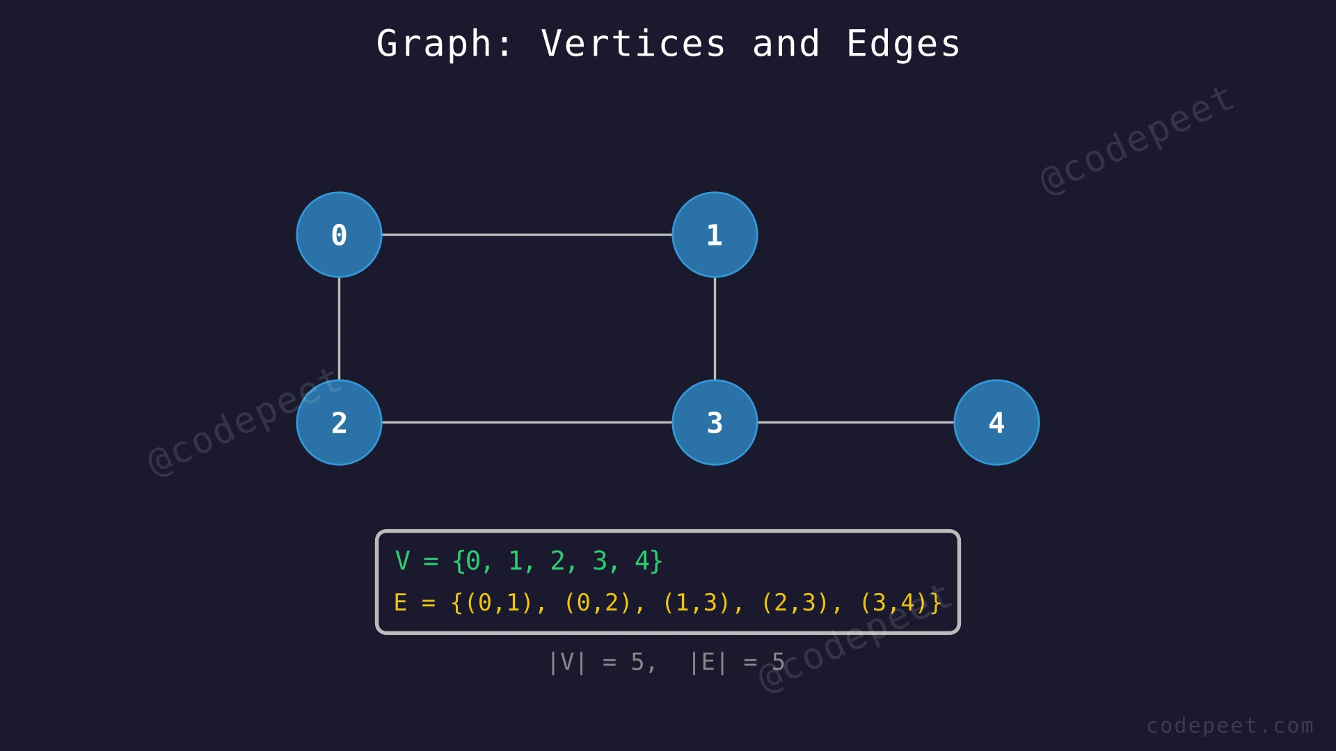
Input: V = 5, edges = [(0,1), (0,2), (1,3), (2,3), (3,4)], undirected
Output (Adjacency List):
0 → [1, 2]
1 → [0, 3]
2 → [0, 3]
3 → [1, 2, 4]
4 → [3]
Explanation: This is an undirected, unweighted graph with 5 vertices and 5 edges. Vertex 3 has the highest degree (3 neighbors: 1, 2, and 4). Vertex 4 has the lowest degree (1 neighbor: 3). Since the graph is undirected, every edge appears in both directions — for instance, edge (0,1) means 1 appears in the neighbor list of 0, and 0 appears in the neighbor list of 1.
Example 2
Input: V = 4, edges = [(0,1,5), (0,2,3), (1,3,2), (2,3,7)], directed and weighted
Output (Adjacency List with Weights):
0 → [(1, w=5), (2, w=3)]
1 → [(3, w=2)]
2 → [(3, w=7)]
3 → []
Explanation: This is a directed, weighted graph. Each edge has a direction and a weight. Edge (0,1,5) means there is an edge from vertex 0 to vertex 1 with weight 5, but NOT from 1 to 0. Vertex 3 has in-degree 2 (edges coming from 1 and 2) but out-degree 0 (no outgoing edges). The shortest path from 0 to 3 goes through vertex 1: 0→1 (cost 5) + 1→3 (cost 2) = total cost 7, which is cheaper than 0→2 (cost 3) + 2→3 (cost 7) = total cost 10.
Example 3
Input: V = 6, edges = [(0,1), (1,2), (3,4)], undirected
Output (Adjacency List):
0 → [1]
1 → [0, 2]
2 → [1]
3 → [4]
4 → [3]
5 → []
Explanation: This is a disconnected graph with three connected components: {0, 1, 2}, {3, 4}, and {5}. Vertex 5 is an isolated vertex with no edges. There is no path from vertex 0 to vertex 3, or from any vertex to vertex 5. The graph has 6 vertices but only 3 edges, making it a sparse graph.
Constraints
- 1 ≤ V ≤ 10^5 (number of vertices)
- 0 ≤ E ≤ min(V × (V − 1) / 2, 10^5) for undirected graphs
- 0 ≤ E ≤ min(V × (V − 1), 10^5) for directed graphs
- Vertices are labeled 0 to V − 1
- The graph may be directed or undirected
- The graph may be weighted or unweighted
- The graph may contain cycles
- The graph may be disconnected
- No self-loops or parallel edges (simple graph) unless otherwise specified
Editorial
Brute Force
Intuition
The simplest way to store a graph is to keep a flat list of all its edges. Think of it like writing down every friendship on a single sheet of paper:
- Alice — Bob
- Alice — Carol
- Bob — Dave
To add a friendship, you just write a new line. To check if two people are friends, you read through the entire list looking for their names together. To find all of Alice's friends, you scan every single line checking if Alice appears in it.
This is called an Edge List representation. It is straightforward to build and uses minimal memory — just one entry per edge. However, finding information requires scanning through every edge in the list, which becomes slow as the graph grows.
Step-by-Step Explanation
Let's trace through building an edge list for the graph from Example 1: V=5, edges = [(0,1), (0,2), (1,3), (2,3), (3,4)], then query it to find the neighbors of vertex 3.
Building the Edge List:
Step 1: Start with an empty edge list.
- edge_list = []
Step 2: Add edge (0,1). Append to the list.
- edge_list = [(0,1)]
Step 3: Add edge (0,2). Append to the list.
- edge_list = [(0,1), (0,2)]
Step 4: Add edge (1,3). Append to the list.
- edge_list = [(0,1), (0,2), (1,3)]
Step 5: Add edge (2,3). Append to the list.
- edge_list = [(0,1), (0,2), (1,3), (2,3)]
Step 6: Add edge (3,4). Append to the list.
- edge_list = [(0,1), (0,2), (1,3), (2,3), (3,4)]
Querying: Find all neighbors of vertex 3
Step 7: Start scanning from the beginning. Check edge (0,1).
- Does edge (0,1) contain vertex 3? No. Skip.
Step 8: Check edge (0,2).
- Does edge (0,2) contain vertex 3? No. Skip.
Step 9: Check edge (1,3).
- Does edge (1,3) contain vertex 3? Yes! The other endpoint is 1.
- neighbors = [1]
Step 10: Check edge (2,3).
- Does edge (2,3) contain vertex 3? Yes! The other endpoint is 2.
- neighbors = [1, 2]
Step 11: Check edge (3,4).
- Does edge (3,4) contain vertex 3? Yes! The other endpoint is 4.
- neighbors = [1, 2, 4]
Step 12: All edges scanned. Result: neighbors of vertex 3 are [1, 2, 4]. We had to check all 5 edges to find 3 neighbors.
Edge List — Build and Query for Neighbors of Vertex 3 — Watch how edges are appended one by one to a flat list, then see how finding neighbors requires scanning every single edge.
Algorithm
Building the Edge List:
- Create an empty list to store edges
- For each edge (u, v), append the pair to the list
Querying Neighbors of Vertex u:
- Initialize an empty result list
- For each edge (a, b) in the edge list:
- If a == u, add b to the result
- Else if b == u (for undirected graphs), add a to the result
- Return the result
Checking if Edge (u, v) Exists:
- For each edge (a, b) in the edge list:
- If (a == u and b == v) or (b == u and a == v for undirected), return true
- Return false
Code
#include <vector>
#include <iostream>
using namespace std;

class EdgeListGraph {
    int V;
    vector<pair<int, int>> edges;
public:
    EdgeListGraph(int v) : V(v) {}

    void addEdge(int u, int v) {
        edges.push_back({u, v});
    }

    bool hasEdge(int u, int v) {
        for (auto& e : edges) {
            if ((e.first == u && e.second == v) ||
                (e.first == v && e.second == u))
                return true;
        }
        return false;
    }

    vector<int> getNeighbors(int u) {
        vector<int> result;
        for (auto& e : edges) {
            if (e.first == u) result.push_back(e.second);
            else if (e.second == u) result.push_back(e.first);
        }
        return result;
    }

    void printGraph() {
        cout << "Edge List:" << endl;
        for (auto& e : edges) {
            cout << e.first << " -- " << e.second << endl;
        }
    }
};
class EdgeListGraph:
def __init__(self, v: int):
self.V = v
self.edges = []
def add_edge(self, u: int, v: int):
self.edges.append((u, v))
def has_edge(self, u: int, v: int) -> bool:
for a, b in self.edges:
if (a == u and b == v) or (a == v and b == u):
return True
return False
def get_neighbors(self, u: int) -> list:
result = []
for a, b in self.edges:
if a == u:
result.append(b)
elif b == u:
result.append(a)
return result
def print_graph(self):
print("Edge List:")
for u, v in self.edges:
print(f"{u} -- {v}")import java.util.*;
class EdgeListGraph {
int V;
List<int[]> edges;
EdgeListGraph(int v) {
this.V = v;
this.edges = new ArrayList<>();
}
void addEdge(int u, int v) {
edges.add(new int[]{u, v});
}
boolean hasEdge(int u, int v) {
for (int[] e : edges) {
if ((e[0] == u && e[1] == v) ||
(e[0] == v && e[1] == u))
return true;
}
return false;
}
List<Integer> getNeighbors(int u) {
List<Integer> result = new ArrayList<>();
for (int[] e : edges) {
if (e[0] == u) result.add(e[1]);
else if (e[1] == u) result.add(e[0]);
}
return result;
}
void printGraph() {
System.out.println("Edge List:");
for (int[] e : edges) {
System.out.println(e[0] + " -- " + e[1]);
}
}
}Complexity Analysis
Time Complexity:
- Add Edge: O(1) — simply append to the list
- Has Edge: O(E) — must scan the entire edge list in the worst case
- Get Neighbors: O(E) — must scan every edge to find those involving the query vertex
Space Complexity: O(E)
The edge list stores exactly one entry per edge. For an undirected graph, if we store each undirected edge once, the space is O(E). This is the most memory-efficient representation.
The fundamental weakness is that every query operation (checking edges, finding neighbors) requires a linear scan of ALL edges. There is no organizational structure to help us find edges for a specific vertex quickly.
Why This Approach Is Not Efficient
The edge list representation requires O(E) time for both edge existence checks and neighbor lookups. For a dense graph with V = 10^4, we could have up to E = V×(V-1)/2 ≈ 5×10^7 edges. Scanning all of them for every single query is far too slow for any algorithm that makes repeated graph queries.
Consider running BFS or DFS, which requires finding all neighbors of each vertex visited. If we use an edge list, finding neighbors of one vertex costs O(E), and since we visit up to V vertices, BFS/DFS alone would cost O(V × E) = O(V² × E / V) which is much worse than necessary.
The root problem: edges are stored in a flat, unorganized list. There is no way to quickly access edges associated with a specific vertex. We need a representation that organizes edges by vertex so that neighbor lookups are faster.
The adjacency matrix solves the edge-checking problem by allowing O(1) edge lookups using a 2D array indexed by vertex pairs.
Better Approach - Adjacency Matrix
Intuition
Instead of a flat list of edges, imagine a spreadsheet where both the rows and columns are labeled with vertex names. Each cell tells you whether an edge exists between the row vertex and the column vertex.
For example, if you want to know whether vertex 2 is connected to vertex 3, you look at row 2, column 3. If the cell contains a 1, they are connected. If it contains a 0, they are not.
This is called an Adjacency Matrix — a V × V grid (2D array) where:
- matrix[i][j] = 1 means there is an edge from vertex i to vertex j
- matrix[i][j] = 0 means there is no edge
For weighted graphs, instead of 1, you store the weight of the edge.
The major advantage is O(1) edge checking — just look up one cell. The trade-off is that the matrix always uses O(V²) space regardless of how many edges actually exist, which is wasteful for sparse graphs.
Step-by-Step Explanation
Let's build an adjacency matrix for the same graph: V=5, edges = [(0,1), (0,2), (1,3), (2,3), (3,4)], then query neighbors of vertex 3.
Building the Matrix:
Step 1: Create a 5×5 matrix filled with zeros.
Step 2: Add edge (0,1): set matrix[0][1] = 1 and matrix[1][0] = 1.
Step 3: Add edge (0,2): set matrix[0][2] = 1 and matrix[2][0] = 1.
Step 4: Add edge (1,3): set matrix[1][3] = 1 and matrix[3][1] = 1.
Step 5: Add edge (2,3): set matrix[2][3] = 1 and matrix[3][2] = 1.
Step 6: Add edge (3,4): set matrix[3][4] = 1 and matrix[4][3] = 1.
Querying: Find all neighbors of vertex 3 (scan row 3)
Step 7: Check matrix[3][0] = 0 → vertex 0 is NOT a neighbor.
Step 8: Check matrix[3][1] = 1 → vertex 1 IS a neighbor! neighbors = [1]
Step 9: Check matrix[3][2] = 1 → vertex 2 IS a neighbor! neighbors = [1, 2]
Step 10: Check matrix[3][3] = 0 → vertex 3 is not its own neighbor (no self-loop).
Step 11: Check matrix[3][4] = 1 → vertex 4 IS a neighbor! neighbors = [1, 2, 4]
Step 12: Row 3 fully scanned. We checked V=5 cells (one per vertex) instead of E=5 edges. For sparse graphs where E is much less than V², this is similar. But for edge checking, matrix[u][v] is O(1) — a massive improvement over the edge list.
Adjacency Matrix — Build and Query Row for Vertex 3 — Watch the 5×5 matrix fill up as edges are added, then see how finding neighbors means scanning a single row.
Algorithm
Building the Adjacency Matrix:
- Create a V × V matrix initialized to all zeros
- For each edge (u, v):
- Set matrix[u][v] = 1
- Set matrix[v][u] = 1 (for undirected graphs)
Checking if Edge (u, v) Exists:
- Return matrix[u][v] == 1
Finding All Neighbors of Vertex u:
- Initialize an empty result list
- For each column j from 0 to V-1:
- If matrix[u][j] == 1, add j to the result
- Return the result
Code
#include <vector>
#include <iostream>
using namespace std;

class AdjMatrixGraph {
    int V;
    vector<vector<int>> matrix;
public:
    AdjMatrixGraph(int v) : V(v), matrix(v, vector<int>(v, 0)) {}

    void addEdge(int u, int v) {
        matrix[u][v] = 1;
        matrix[v][u] = 1;
    }

    bool hasEdge(int u, int v) {
        return matrix[u][v] == 1;
    }

    vector<int> getNeighbors(int u) {
        vector<int> result;
        for (int v = 0; v < V; v++) {
            if (matrix[u][v] == 1) {
                result.push_back(v);
            }
        }
        return result;
    }

    void printGraph() {
        cout << "Adjacency Matrix:" << endl;
        for (int i = 0; i < V; i++) {
            for (int j = 0; j < V; j++) {
                cout << matrix[i][j] << " ";
            }
            cout << endl;
        }
    }
};
class AdjMatrixGraph:
def __init__(self, v: int):
self.V = v
self.matrix = [[0] * v for _ in range(v)]
def add_edge(self, u: int, v: int):
self.matrix[u][v] = 1
self.matrix[v][u] = 1
def has_edge(self, u: int, v: int) -> bool:
return self.matrix[u][v] == 1
def get_neighbors(self, u: int) -> list:
result = []
for v in range(self.V):
if self.matrix[u][v] == 1:
result.append(v)
return result
def print_graph(self):
print("Adjacency Matrix:")
for row in self.matrix:
print(" ".join(str(x) for x in row))import java.util.*;
class AdjMatrixGraph {
int V;
int[][] matrix;
AdjMatrixGraph(int v) {
this.V = v;
this.matrix = new int[v][v];
}
void addEdge(int u, int v) {
matrix[u][v] = 1;
matrix[v][u] = 1;
}
boolean hasEdge(int u, int v) {
return matrix[u][v] == 1;
}
List<Integer> getNeighbors(int u) {
List<Integer> result = new ArrayList<>();
for (int v = 0; v < V; v++) {
if (matrix[u][v] == 1) {
result.add(v);
}
}
return result;
}
void printGraph() {
System.out.println("Adjacency Matrix:");
for (int i = 0; i < V; i++) {
for (int j = 0; j < V; j++) {
System.out.print(matrix[i][j] + " ");
}
System.out.println();
}
}
}Complexity Analysis
Time Complexity:
- Add Edge: O(1) — just set two cells in the matrix
- Has Edge: O(1) — direct array lookup at matrix[u][v]
- Get Neighbors: O(V) — must scan the entire row of V cells
Space Complexity: O(V²)
The matrix always occupies V × V space regardless of the number of edges. For a graph with V = 10^4, the matrix requires 10^8 cells — about 100 MB of memory even if the graph has only a few edges.
The adjacency matrix trades space for speed on edge existence checks. It achieves O(1) edge lookup (a massive improvement over edge list's O(E)), but neighbor finding is still O(V) because we must scan the entire row. For sparse graphs, most of the V cells in any row will be zeros, wasting both memory and query time.
Why This Approach Is Not Efficient
The adjacency matrix uses O(V²) space, which is wasteful for sparse graphs. A social network with V = 10^5 users where each person has on average 100 friends (E ≈ 5 × 10^6) would require a matrix of 10^10 cells — roughly 10 GB of memory — even though only 10^7 out of those 10^10 cells would be non-zero.
Finding neighbors takes O(V) time because you scan an entire row. In a sparse graph where a vertex has only 3 neighbors out of 10^5 possible vertices, you waste 99,997 cell checks on zeros.
For graph algorithms like BFS and DFS that iterate over the neighbors of each visited vertex, the adjacency matrix gives O(V²) traversal time (scanning all V cells for each of V vertices), regardless of how few edges exist. A sparse graph with E = O(V) edges should allow traversal in O(V + E) = O(V) time, not O(V²).
We need a representation that stores only the edges that exist while still allowing fast neighbor access. The adjacency list achieves this by maintaining a separate list of neighbors for each vertex.
Optimal Approach - Adjacency List
Intuition
Instead of a massive V × V grid where most cells are empty, we give each vertex its own personal contact list containing only its actual neighbors.
Think of it like a phone book organized by person. Under "Alice" you see only her actual contacts: Bob, Carol. Under "Bob" you see: Alice, Dave. You do not waste pages listing every person Alice is NOT connected to.
This is the Adjacency List representation — an array of V lists, where the list at index i contains all vertices that are neighbors of vertex i.
Why this is optimal for most use cases:
- Space-efficient: Stores only edges that exist → O(V + E) space
- Fast neighbor iteration: To find all neighbors of vertex u, just traverse adj[u] → O(degree(u)) time
- BFS/DFS optimal: Traversal visits each vertex and each edge once → O(V + E) total
- Flexible: Easily adapted for weighted, directed, and undirected graphs
The only trade-off compared to the adjacency matrix is that checking whether a specific edge (u, v) exists requires scanning u's neighbor list, taking O(degree(u)) instead of O(1). But for the vast majority of graph algorithms, iterating over neighbors is far more common than checking specific edge existence.
Step-by-Step Explanation
Let's build an adjacency list for V=5, edges = [(0,1), (0,2), (1,3), (2,3), (3,4)], then query neighbors of vertex 3.
Building the Adjacency List:
Step 1: Create 5 empty lists, one for each vertex.
- adj[0] = [], adj[1] = [], adj[2] = [], adj[3] = [], adj[4] = []
Step 2: Add edge (0,1): append 1 to adj[0] and 0 to adj[1].
- adj[0] = [1], adj[1] = [0]
Step 3: Add edge (0,2): append 2 to adj[0] and 0 to adj[2].
- adj[0] = [1, 2], adj[2] = [0]
Step 4: Add edge (1,3): append 3 to adj[1] and 1 to adj[3].
- adj[1] = [0, 3], adj[3] = [1]
Step 5: Add edge (2,3): append 3 to adj[2] and 2 to adj[3].
- adj[2] = [0, 3], adj[3] = [1, 2]
Step 6: Add edge (3,4): append 4 to adj[3] and 3 to adj[4].
- adj[3] = [1, 2, 4], adj[4] = [3]
Step 7: All edges processed. Complete adjacency list:
- adj[0] = [1, 2], adj[1] = [0, 3], adj[2] = [0, 3], adj[3] = [1, 2, 4], adj[4] = [3]
Querying: Find all neighbors of vertex 3
Step 8: Access adj[3] directly — no scanning needed.
- adj[3] = [1, 2, 4]
Step 9: Result: neighbors of vertex 3 are [1, 2, 4]. We accessed the list in O(1) and iterated through 3 elements (the degree of vertex 3). Compare this to edge list's O(E)=O(5) full scan and adjacency matrix's O(V)=O(5) row scan.
Adjacency List — Build Graph and Query Neighbors Instantly — Watch edges being added to the graph structure one by one, then see how querying neighbors of vertex 3 is an instant direct access.
Algorithm
Building the Adjacency List:
- Create an array of V empty lists
- For each edge (u, v):
- Append v to adj[u]
- Append u to adj[v] (for undirected graphs)
Finding All Neighbors of Vertex u:
- Return adj[u] (direct access)
Checking if Edge (u, v) Exists:
- Search for v in adj[u]
- If found, return true; otherwise, return false
Note: For weighted graphs, store pairs (neighbor, weight) instead of just neighbor values.
Code
#include <vector>
#include <iostream>
using namespace std;

class AdjListGraph {
    int V;
    vector<vector<int>> adj;
public:
    AdjListGraph(int v) : V(v), adj(v) {}

    void addEdge(int u, int v) {
        adj[u].push_back(v);
        adj[v].push_back(u);
    }

    bool hasEdge(int u, int v) {
        for (int neighbor : adj[u]) {
            if (neighbor == v) return true;
        }
        return false;
    }

    vector<int> getNeighbors(int u) {
        return adj[u];
    }

    void printGraph() {
        cout << "Adjacency List:" << endl;
        for (int i = 0; i < V; i++) {
            cout << i << " -> ";
            for (int neighbor : adj[i]) {
                cout << neighbor << " ";
            }
            cout << endl;
        }
    }
};
class AdjListGraph:
def __init__(self, v: int):
self.V = v
self.adj = [[] for _ in range(v)]
def add_edge(self, u: int, v: int):
self.adj[u].append(v)
self.adj[v].append(u)
def has_edge(self, u: int, v: int) -> bool:
return v in self.adj[u]
def get_neighbors(self, u: int) -> list:
return self.adj[u]
def print_graph(self):
print("Adjacency List:")
for i in range(self.V):
neighbors = " ".join(str(n) for n in self.adj[i])
print(f"{i} -> {neighbors}")import java.util.*;
class AdjListGraph {
int V;
List<List<Integer>> adj;
AdjListGraph(int v) {
this.V = v;
this.adj = new ArrayList<>();
for (int i = 0; i < v; i++) {
adj.add(new ArrayList<>());
}
}
void addEdge(int u, int v) {
adj.get(u).add(v);
adj.get(v).add(u);
}
boolean hasEdge(int u, int v) {
return adj.get(u).contains(v);
}
List<Integer> getNeighbors(int u) {
return adj.get(u);
}
void printGraph() {
System.out.println("Adjacency List:");
for (int i = 0; i < V; i++) {
System.out.print(i + " -> ");
for (int neighbor : adj.get(i)) {
System.out.print(neighbor + " ");
}
System.out.println();
}
}
}Complexity Analysis
Time Complexity:
- Add Edge: O(1) — append to two lists
- Has Edge: O(degree(u)) — scan u's neighbor list. In the worst case (complete graph), this is O(V), but for sparse graphs it is O(average_degree) which is typically much smaller
- Get Neighbors: O(1) for access + O(degree(u)) to iterate — you get only the actual neighbors, with no wasted checks on non-neighbors
- BFS/DFS Traversal: O(V + E) — each vertex is visited once, and each edge is examined once
Space Complexity: O(V + E)
We store V lists (one per vertex) plus a total of 2E entries across all lists (each undirected edge is stored in two lists). This is optimal because we store only the information that actually exists — no wasted space on absent edges.
Comparison Summary:
| Operation | Edge List | Adj. Matrix | Adj. List |
|---|---|---|---|
| Space | O(E) | O(V²) | O(V + E) |
| Add Edge | O(1) | O(1) | O(1) |
| Has Edge | O(E) | O(1) | O(degree) |
| Neighbors | O(E) | O(V) | O(degree) |
| BFS/DFS | O(V × E) | O(V²) | O(V + E) |
The adjacency list is the most widely used graph representation because it provides the best balance of space efficiency and fast neighbor iteration, which is the operation most graph algorithms rely on. The adjacency matrix is preferred only when edge existence checks dominate (e.g., dense graph algorithms) or when V is small enough that O(V²) space is acceptable.