Dijkstra's Algorithm
Description
Given an undirected, weighted, connected graph with V vertices numbered 0 to V-1 and E edges, and a source vertex src, find the shortest distance from src to every other vertex.
You are given:
V: the number of verticesedges[][]: a 2D array where each entry[u, v, w]represents an undirected edge between vertexuand vertexvwith weightwsrc: the source vertex
Return an array dist[] of size V where dist[i] is the shortest distance from src to vertex i.
The graph is connected (every vertex is reachable from every other vertex) and contains no negative weight edges. The non-negative weight constraint is crucial — it allows a greedy approach where once a vertex's shortest distance is finalized, it never needs to be updated again.
Examples
Example 1
Input: V = 3, edges = [[0,1,1], [1,2,3], [0,2,6]], src = 2
Graph:
0 ---(1)--- 1
|           |
+---(6)-----+---(3)--- 2
Output: [4, 3, 0]
Explanation:
- dist[2] = 0 (source vertex)
- dist[1] = 3 (direct edge 2—1 with weight 3)
- dist[0] = 4 (path 2→1→0, weight 3+1=4. The direct edge 2→0 costs 6, which is longer)
Example 2
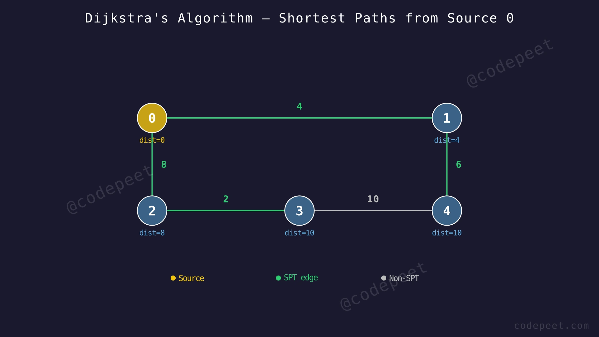
Input: V = 5, edges = [[0,1,4], [0,2,8], [1,4,6], [2,3,2], [3,4,10]], src = 0
Graph:
0 ---(4)--- 1
|           |
(8)        (6)
|           |
2 ---(2)--- 3 ---(10)--- 4
Output: [0, 4, 8, 10, 10]
Explanation:
- dist[0] = 0 (source vertex)
- dist[1] = 4 (direct edge 0→1, weight 4)
- dist[2] = 8 (direct edge 0→2, weight 8)
- dist[3] = 10 (path 0→2→3, weight 8+2=10)
- dist[4] = 10 (path 0→1→4, weight 4+6=10. The path 0→2→3→4 costs 8+2+10=20, which is longer)
Example 3
Input: V = 4, edges = [[0,1,5], [0,2,1], [2,1,2], [1,3,1], [2,3,7]], src = 0
Output: [0, 3, 1, 4]
Explanation:
- dist[0] = 0 (source)
- dist[2] = 1 (direct edge 0→2, weight 1)
- dist[1] = 3 (path 0→2→1, weight 1+2=3. The direct edge 0→1 costs 5, which is longer)
- dist[3] = 4 (path 0→2→1→3, weight 1+2+1=4. The path 0→2→3 costs 1+7=8, which is longer)
This example shows how Dijkstra finds that going through more edges can be cheaper than direct routes.
Constraints
- 1 ≤ V ≤ 10^6
- 1 ≤ E = edges.size() ≤ 10^6
- 0 ≤ edges[i][0], edges[i][1] ≤ V - 1
- 0 ≤ edges[i][2] ≤ 10^4
- 0 ≤ src < V
- The graph is connected
- The graph does not contain negative weight edges
- All shortest distances fit in a 32-bit integer
Editorial
Brute Force
Intuition
The most straightforward way to find shortest distances is to enumerate every possible simple path from the source to each destination and record the minimum cost.
A "simple path" is one that doesn't visit the same vertex twice (this prevents infinite loops in undirected graphs with cycles). For each path from src to some vertex v, we compute the total edge weight. The shortest distance to v is the minimum across all such paths.
We can enumerate simple paths using DFS with backtracking: maintain a visited set for the current path, explore each unvisited neighbor, and when we reach a vertex, update its shortest distance if the current path cost is less. After exploring, we backtrack by removing the vertex from the visited set.
The problem: the number of simple paths in a graph can be factorial — up to O(V!) in the worst case. A complete graph on V vertices has an astronomical number of paths between any two vertices. For V ≤ 10^6, this is completely infeasible.
Step-by-Step Explanation
Let's trace with V = 5, edges = [[0,1,4],[0,2,8],[1,4,6],[2,3,2],[3,4,10]], src = 0.
Step 1: Initialize dist = [0, ∞, ∞, ∞, ∞]. Start DFS from vertex 0 with cost 0 and visited = {0}.
Step 2: At vertex 0. Explore neighbor 1 (weight 4). Cost = 0+4 = 4 < ∞. Update dist[1] = 4. Add 1 to visited. Recurse.
Step 3: At vertex 1. Explore neighbor 4 (weight 6). Cost = 4+6 = 10 < ∞. Update dist[4] = 10. Add 4 to visited. Recurse.
Step 4: At vertex 4. Explore neighbor 3 (weight 10). Cost = 10+10 = 20 < ∞. Update dist[3] = 20. Add 3 to visited. Recurse.
Step 5: At vertex 3. Explore neighbor 2 (weight 2). Cost = 20+2 = 22 < ∞. Update dist[2] = 22. Add 2 to visited. Recurse.
Step 6: At vertex 2. Neighbor 0 is visited, neighbor 3 is visited. Dead end. Backtrack: remove 2 from visited. Backtrack from 3 (remove 3), from 4 (remove 4), from 1 (remove 1).
Step 7: Back at vertex 0. Explore neighbor 2 (weight 8). Cost = 0+8 = 8 < 22. Update dist[2] = 8. Add 2 to visited. Recurse.
Step 8: At vertex 2. Explore neighbor 3 (weight 2). Cost = 8+2 = 10 < 20. Update dist[3] = 10. Recurse into 3.
Step 9: At vertex 3. Explore neighbor 4 (weight 10). Cost = 10+10 = 20 > 10. No improvement to dist[4]. Still explore for completeness but no update.
Step 10: All paths explored. Final dist = [0, 4, 8, 10, 10].
Result: [0, 4, 8, 10, 10]. We explored multiple paths and found improvements along the way.
DFS All Simple Paths — Exhaustive Path Enumeration — Watch DFS explore every simple path from source vertex 0, maintaining a per-path visited set to avoid cycles. Distances are updated whenever a cheaper path is found.
Algorithm
- Build an adjacency list from the edges array (undirected — add both directions).
- Initialize
dist[]with ∞ for all vertices. Setdist[src] = 0. - Define a recursive DFS function
dfs(u, cost, path_visited):
a. For each neighborvofuwith edge weightw:- If
vis not inpath_visited:- If
cost + w < dist[v], updatedist[v] = cost + w. - Add
vtopath_visited. - Recursively call
dfs(v, cost + w, path_visited). - Remove
vfrompath_visited(backtrack).
- If
- If
- Call
dfs(src, 0, {src}). - Return
dist[].
Code
class Solution {
public:
    void dfs(int u, int cost, vector<vector<pair<int,int>>>& adj,
             vector<int>& dist, vector<bool>& pathVisited) {
        for (auto& [v, w] : adj[u]) {
            if (!pathVisited[v]) {
                if (cost + w < dist[v]) {
                    dist[v] = cost + w;
                }
                pathVisited[v] = true;
                dfs(v, cost + w, adj, dist, pathVisited);
                pathVisited[v] = false; // backtrack
            }
        }
    }

    vector<int> dijkstra(int V, vector<vector<int>>& edges, int src) {
        vector<vector<pair<int,int>>> adj(V);
        for (auto& e : edges) {
            adj[e[0]].push_back({e[1], e[2]});
            adj[e[1]].push_back({e[0], e[2]});
        }

        vector<int> dist(V, INT_MAX);
        dist[src] = 0;

        vector<bool> pathVisited(V, false);
        pathVisited[src] = true;
        dfs(src, 0, adj, dist, pathVisited);

        return dist;
    }
};
class Solution:
def dijkstra(self, V, edges, src):
adj = [[] for _ in range(V)]
for u, v, w in edges:
adj[u].append((v, w))
adj[v].append((u, w))
dist = [float('inf')] * V
dist[src] = 0
def dfs(u, cost, path_visited):
for v, w in adj[u]:
if v not in path_visited:
if cost + w < dist[v]:
dist[v] = cost + w
path_visited.add(v)
dfs(v, cost + w, path_visited)
path_visited.remove(v) # backtrack
dfs(src, 0, {src})
return distclass Solution {
public int[] dijkstra(int V, int[][] edges, int src) {
List<List<int[]>> adj = new ArrayList<>();
for (int i = 0; i < V; i++) adj.add(new ArrayList<>());
for (int[] e : edges) {
adj.get(e[0]).add(new int[]{e[1], e[2]});
adj.get(e[1]).add(new int[]{e[0], e[2]});
}
int[] dist = new int[V];
Arrays.fill(dist, Integer.MAX_VALUE);
dist[src] = 0;
boolean[] pathVisited = new boolean[V];
pathVisited[src] = true;
dfs(src, 0, adj, dist, pathVisited);
return dist;
}
private void dfs(int u, int cost, List<List<int[]>> adj,
int[] dist, boolean[] pathVisited) {
for (int[] edge : adj.get(u)) {
int v = edge[0], w = edge[1];
if (!pathVisited[v]) {
if (cost + w < dist[v]) {
dist[v] = cost + w;
}
pathVisited[v] = true;
dfs(v, cost + w, adj, dist, pathVisited);
pathVisited[v] = false; // backtrack
}
}
}
}Complexity Analysis
Time Complexity: O(V!) in the worst case
In a complete graph (every vertex connected to every other vertex), the number of simple paths from source to any vertex is O(V!). For each path, we do O(1) work per edge. With V ≤ 10^6, this is astronomically slow.
Even for moderate V (say V = 20), there are already trillions of possible paths. This approach is only feasible for very small graphs (V ≤ 10-15).
Space Complexity: O(V + E)
- O(V + E) for the adjacency list.
- O(V) for the distance array and path-visited array.
- O(V) for the recursion stack.
Why This Approach Is Not Efficient
The brute force explores every possible path, but most of this exploration is wasted. The fundamental insight we're missing is:
Greedy Principle: If all edge weights are non-negative, the vertex with the smallest current distance from the source will NEVER have its distance reduced further.
Why? Because any other path to this vertex must go through vertices that are farther away (or equally far), and adding more non-negative edges can only increase the total distance.
This means we can finalize vertices one by one: always pick the unfinalized vertex with the smallest distance, mark it as finalized, and update its neighbors. Once finalized, we never look at a vertex again. This is the core of Dijkstra's algorithm — a greedy approach that processes each vertex at most once, avoiding the factorial explosion of path enumeration.
Better Approach - Dijkstra with Linear Scan
Intuition
Dijkstra's algorithm uses a greedy strategy: repeatedly pick the unvisited vertex with the smallest known distance, finalize it, and update its neighbors.
The key insight is that with non-negative edge weights, the vertex with the smallest tentative distance is guaranteed to have its final shortest distance. No future path through other vertices can beat it, because those vertices are farther away and adding non-negative weights only increases the total.
Think of it like a spreading wavefront of water on a surface. Water spreads outward from the source, always reaching the nearest unflooded point first. Once a point is flooded, its distance (time to reach) is finalized — water can't arrive faster from a longer route.
In this "Better" version, we find the minimum-distance unvisited vertex using a linear scan through all vertices. This takes O(V) per extraction and O(V) extractions = O(V²) total. This is efficient for dense graphs (where E ≈ V²) but becomes a bottleneck for sparse graphs (where E ≈ V).
Step-by-Step Explanation
Let's trace with V = 5, edges = [[0,1,4],[0,2,8],[1,4,6],[2,3,2],[3,4,10]], src = 0.
Step 1: Initialize dist = [0, ∞, ∞, ∞, ∞]. Finalized = {} (empty set).
Step 2: Find minimum unfinalized vertex: vertex 0 (dist=0). Finalize vertex 0.
Relax neighbors:
- 0→1(4): dist[1] = min(∞, 0+4) = 4. Updated!
- 0→2(8): dist[2] = min(∞, 0+8) = 8. Updated!
dist = [0, 4, 8, ∞, ∞]
Step 3: Find minimum unfinalized: vertex 1 (dist=4). Finalize vertex 1.
Relax neighbors:
- 1→0(4): vertex 0 already finalized. Skip.
- 1→4(6): dist[4] = min(∞, 4+6) = 10. Updated!
dist = [0, 4, 8, ∞, 10]
Step 4: Find minimum unfinalized: vertex 2 (dist=8). Finalize vertex 2.
Relax neighbors:
- 2→0(8): already finalized. Skip.
- 2→3(2): dist[3] = min(∞, 8+2) = 10. Updated!
dist = [0, 4, 8, 10, 10]
Step 5: Find minimum unfinalized: vertex 3 (dist=10, tie with vertex 4 — pick either). Finalize vertex 3.
Relax neighbors:
- 3→2(2): already finalized. Skip.
- 3→4(10): dist[4] = min(10, 10+10) = 10. No change.
dist = [0, 4, 8, 10, 10]
Step 6: Find minimum unfinalized: vertex 4 (dist=10). Finalize vertex 4.
Relax neighbors:
- 4→1(6): already finalized. Skip.
- 4→3(10): already finalized. Skip.
Result: [0, 4, 8, 10, 10]. All vertices finalized.
Dijkstra's Algorithm (O(V²)) — Greedy Vertex Selection — Watch Dijkstra's greedy strategy: in each step, the unvisited vertex with the smallest distance is finalized and its neighbors are updated. The 'wavefront' of finalized vertices expands outward from the source.
Algorithm
- Build an adjacency list from the edges (add both directions since the graph is undirected).
- Initialize
dist[]with ∞ for all vertices. Setdist[src] = 0. - Create a
finalized[]boolean array, all set tofalse. - Repeat V times:
a. Find minimum: Scan all V vertices to find the unfinalized vertexuwith the smallestdist[u].
b. Finalize: Markuas finalized.
c. Relax neighbors: For each neighborvofuwith edge weightw:- If
vis not finalized anddist[u] + w < dist[v]:- Update
dist[v] = dist[u] + w.
- Update
- If
- Return
dist[].
Code
class Solution {
public:
    vector<int> dijkstra(int V, vector<vector<int>>& edges, int src) {
        vector<vector<pair<int,int>>> adj(V);
        for (auto& e : edges) {
            adj[e[0]].push_back({e[1], e[2]});
            adj[e[1]].push_back({e[0], e[2]});
        }

        vector<int> dist(V, INT_MAX);
        vector<bool> finalized(V, false);
        dist[src] = 0;

        for (int i = 0; i < V; i++) {
            // Find unfinalized vertex with minimum distance
            int u = -1;
            for (int j = 0; j < V; j++) {
                if (!finalized[j] && (u == -1 || dist[j] < dist[u])) {
                    u = j;
                }
            }

            if (dist[u] == INT_MAX) break; // Remaining vertices unreachable
            finalized[u] = true;

            // Relax neighbors
            for (auto& [v, w] : adj[u]) {
                if (!finalized[v] && dist[u] + w < dist[v]) {
                    dist[v] = dist[u] + w;
                }
            }
        }

        return dist;
    }
};
class Solution:
def dijkstra(self, V, edges, src):
adj = [[] for _ in range(V)]
for u, v, w in edges:
adj[u].append((v, w))
adj[v].append((u, w))
dist = [float('inf')] * V
finalized = [False] * V
dist[src] = 0
for _ in range(V):
# Find unfinalized vertex with minimum distance
u = -1
for j in range(V):
if not finalized[j] and (u == -1 or dist[j] < dist[u]):
u = j
if dist[u] == float('inf'):
break # Remaining vertices unreachable
finalized[u] = True
# Relax neighbors
for v, w in adj[u]:
if not finalized[v] and dist[u] + w < dist[v]:
dist[v] = dist[u] + w
return distclass Solution {
public int[] dijkstra(int V, int[][] edges, int src) {
List<List<int[]>> adj = new ArrayList<>();
for (int i = 0; i < V; i++) adj.add(new ArrayList<>());
for (int[] e : edges) {
adj.get(e[0]).add(new int[]{e[1], e[2]});
adj.get(e[1]).add(new int[]{e[0], e[2]});
}
int[] dist = new int[V];
Arrays.fill(dist, Integer.MAX_VALUE);
boolean[] finalized = new boolean[V];
dist[src] = 0;
for (int i = 0; i < V; i++) {
// Find unfinalized vertex with minimum distance
int u = -1;
for (int j = 0; j < V; j++) {
if (!finalized[j] && (u == -1 || dist[j] < dist[u])) {
u = j;
}
}
if (dist[u] == Integer.MAX_VALUE) break;
finalized[u] = true;
// Relax neighbors
for (int[] edge : adj.get(u)) {
int v = edge[0], w = edge[1];
if (!finalized[v] && dist[u] + w < dist[v]) {
dist[v] = dist[u] + w;
}
}
}
return dist;
}
}Complexity Analysis
Time Complexity: O(V²)
The outer loop runs V times. In each iteration:
- Finding the minimum via linear scan: O(V)
- Relaxing all neighbors of the chosen vertex: O(degree of vertex)
Total: V × O(V) + sum of all degrees = O(V²) + O(E) = O(V²).
For dense graphs where E ≈ V², this is optimal. But for sparse graphs where E ≈ V, the O(V²) term dominates unnecessarily.
With V ≤ 10^6, O(V²) = 10^12 operations — this will TLE (Time Limit Exceeded).
Space Complexity: O(V + E)
- O(V + E) for the adjacency list.
- O(V) for the distance array and finalized array.
Why This Approach Is Not Efficient
The O(V²) Dijkstra works correctly and is even optimal for dense graphs, but the bottleneck is the linear scan to find the minimum distance vertex. Each scan costs O(V), and we perform V scans → O(V²) total.
But we only need two operations on the set of unfinalized vertices:
- Extract-Min: Remove and return the vertex with the smallest distance.
- Decrease-Key: Update a vertex's distance to a smaller value.
A min-heap (priority queue) supports both operations in O(log V) time. With a heap:
- V extract-min operations: O(V log V)
- Up to E decrease-key operations: O(E log V)
- Total: O((V + E) log V)
For sparse graphs (E ≈ V): O(V log V) ≪ O(V²)
For the given constraints (V, E ≤ 10^6): O(10^6 × 20) ≈ 2 × 10^7 operations — well within time limits.
Optimal Approach - Dijkstra with Min-Heap (Priority Queue)
Intuition
The optimal implementation of Dijkstra's algorithm replaces the expensive linear scan with a min-heap (priority queue). The heap always gives us the unfinalized vertex with the smallest distance in O(log V) time.
The algorithm works like this:
- Start with only the source in the heap with distance 0.
- Extract the minimum-distance vertex from the heap.
- If we've already processed this vertex (it was extracted before with a smaller distance), skip it.
- Otherwise, relax all its neighbors. For each neighbor whose distance improves, push the new (distance, vertex) pair into the heap.
- Repeat until the heap is empty.
Why push duplicates instead of decrease-key? In many languages, the standard priority queue doesn't support decrease-key efficiently. Instead, we push a new entry whenever a distance improves and rely on the "skip if already processed" check (step 3) to ignore stale entries. This is called the lazy deletion approach.
The heap ensures we always process vertices in order of increasing distance — exactly the greedy order that makes Dijkstra correct. But now, finding the next vertex to process takes O(log V) instead of O(V).
Step-by-Step Explanation
Let's trace with V = 5, edges = [[0,1,4],[0,2,8],[1,4,6],[2,3,2],[3,4,10]], src = 0.
Step 1: Initialize dist = [0, ∞, ∞, ∞, ∞]. Push (0, 0) into min-heap.
Heap: [(0, 0)]
Step 2: Extract min → (0, vertex 0). dist[0]=0, matches. Process vertex 0.
- 0→1(4): dist[1] = 0+4 = 4 < ∞. Update! Push (4, 1).
- 0→2(8): dist[2] = 0+8 = 8 < ∞. Update! Push (8, 2).
dist = [0, 4, 8, ∞, ∞]. Heap: [(4, 1), (8, 2)]
Step 3: Extract min → (4, vertex 1). dist[1]=4, matches. Process vertex 1.
- 1→0(4): dist[0]=0, 4+4=8 > 0. No update.
- 1→4(6): dist[4] = 4+6 = 10 < ∞. Update! Push (10, 4).
dist = [0, 4, 8, ∞, 10]. Heap: [(8, 2), (10, 4)]
Step 4: Extract min → (8, vertex 2). dist[2]=8, matches. Process vertex 2.
- 2→0(8): dist[0]=0, no update.
- 2→3(2): dist[3] = 8+2 = 10 < ∞. Update! Push (10, 3).
dist = [0, 4, 8, 10, 10]. Heap: [(10, 3), (10, 4)]
Step 5: Extract min → (10, vertex 3). dist[3]=10, matches. Process vertex 3.
- 3→2(2): dist[2]=8, 10+2=12 > 8. No update.
- 3→4(10): dist[4]=10, 10+10=20 > 10. No update.
Heap: [(10, 4)]
Step 6: Extract min → (10, vertex 4). dist[4]=10, matches. Process vertex 4.
- 4→1(6): dist[1]=4, 10+6=16 > 4. No update.
- 4→3(10): dist[3]=10, 10+10=20 > 10. No update.
Heap: [] (empty). Done!
Result: [0, 4, 8, 10, 10]
Dijkstra with Min-Heap — O((V+E) log V) Shortest Paths — Watch the priority queue version of Dijkstra. The min-heap always yields the closest unprocessed vertex. Each extraction is O(log V) instead of O(V), making this dramatically faster for large sparse graphs.
Algorithm
- Build an adjacency list from the edges (add both directions).
- Initialize
dist[]with ∞ for all vertices. Setdist[src] = 0. - Create a min-heap (priority queue). Push
(0, src). - While the heap is not empty:
a. Extract the minimum element(d, u)from the heap.
b. Stale check: Ifd > dist[u], this entry is outdated — skip it.
c. For each neighborvofuwith edge weightw:- If
dist[u] + w < dist[v]:- Update
dist[v] = dist[u] + w. - Push
(dist[v], v)into the heap.
- Update
- If
- Return
dist[].
Note on stale entries: When we improve a vertex's distance, we push a new entry into the heap rather than updating the existing one. The old entry remains in the heap but with a larger distance. When we later extract it, the stale check (d > dist[u]) detects it and skips it. This "lazy deletion" approach avoids the need for decrease-key operations.
Code
class Solution {
public:
    vector<int> dijkstra(int V, vector<vector<int>>& edges, int src) {
        // Build adjacency list
        vector<vector<pair<int,int>>> adj(V);
        for (auto& e : edges) {
            adj[e[0]].push_back({e[1], e[2]});
            adj[e[1]].push_back({e[0], e[2]});
        }

        // Distance array initialized to infinity
        vector<int> dist(V, INT_MAX);
        dist[src] = 0;

        // Min-heap: (distance, vertex)
        priority_queue<pair<int,int>, vector<pair<int,int>>, greater<pair<int,int>>> pq;
        pq.push({0, src});

        while (!pq.empty()) {
            auto [d, u] = pq.top();
            pq.pop();

            // Skip stale entries
            if (d > dist[u]) continue;

            // Relax all neighbors
            for (auto& [v, w] : adj[u]) {
                if (dist[u] + w < dist[v]) {
                    dist[v] = dist[u] + w;
                    pq.push({dist[v], v});
                }
            }
        }

        return dist;
    }
};
import heapq
class Solution:
def dijkstra(self, V, edges, src):
# Build adjacency list
adj = [[] for _ in range(V)]
for u, v, w in edges:
adj[u].append((v, w))
adj[v].append((u, w))
# Distance array initialized to infinity
dist = [float('inf')] * V
dist[src] = 0
# Min-heap: (distance, vertex)
heap = [(0, src)]
while heap:
d, u = heapq.heappop(heap)
# Skip stale entries
if d > dist[u]:
continue
# Relax all neighbors
for v, w in adj[u]:
if dist[u] + w < dist[v]:
dist[v] = dist[u] + w
heapq.heappush(heap, (dist[v], v))
return distclass Solution {
public int[] dijkstra(int V, int[][] edges, int src) {
// Build adjacency list
List<List<int[]>> adj = new ArrayList<>();
for (int i = 0; i < V; i++) adj.add(new ArrayList<>());
for (int[] e : edges) {
adj.get(e[0]).add(new int[]{e[1], e[2]});
adj.get(e[1]).add(new int[]{e[0], e[2]});
}
// Distance array initialized to infinity
int[] dist = new int[V];
Arrays.fill(dist, Integer.MAX_VALUE);
dist[src] = 0;
// Min-heap: [distance, vertex]
PriorityQueue<int[]> pq = new PriorityQueue<>((a, b) -> a[0] - b[0]);
pq.offer(new int[]{0, src});
while (!pq.isEmpty()) {
int[] top = pq.poll();
int d = top[0], u = top[1];
// Skip stale entries
if (d > dist[u]) continue;
// Relax all neighbors
for (int[] edge : adj.get(u)) {
int v = edge[0], w = edge[1];
if (dist[u] + w < dist[v]) {
dist[v] = dist[u] + w;
pq.offer(new int[]{dist[v], v});
}
}
}
return dist;
}
}Complexity Analysis
Time Complexity: O((V + E) × log V)
- Heap extractions: At most V vertices are processed (each extracted once for its final distance). Additional stale entries may be extracted but skipped in O(1). Total extractions: O(V + E) in the worst case. Each extraction: O(log(V + E)) = O(log V).
- Heap insertions: At most E insertions (one per edge relaxation). Each insertion: O(log V).
- Total: O((V + E) × log V).
For V = E = 10^6: O(10^6 × 20) ≈ 2 × 10^7 — easily within time limits.
Compare the three approaches:
- Brute Force (DFS all paths): O(V!) — impossible for V > 15
- Dijkstra with linear scan: O(V²) — TLE for V = 10^6
- Dijkstra with min-heap: O((V+E) log V) — optimal for sparse graphs ✓
Space Complexity: O(V + E)
- O(V + E) for the adjacency list.
- O(V) for the distance array.
- O(V + E) for the heap (at most E entries due to lazy deletion).
- Overall: O(V + E).