Number of Operations to Make Network Connected
Description
You are given a network of n computers, labeled from 0 to n - 1. These computers are connected by ethernet cables, where each cable directly links two computers. The connections are represented as a list connections, where connections[i] = [a, b] means there is a cable between computer a and computer b.
Computers can communicate either directly (through a shared cable) or indirectly (through a chain of cables via other computers). However, not all computers may be able to reach each other initially — the network might be split into separate groups (called connected components).
You are allowed to perform the following operation any number of times: remove a cable between two directly connected computers and use that cable to connect any two computers that are not currently connected.
Return the minimum number of operations needed to make every computer able to communicate with every other computer. If it is impossible to connect all computers (because there are not enough cables), return -1.
Key Insight: To connect n computers into a single network, you need at least n - 1 cables. If you have fewer cables than that, it is impossible regardless of how you rearrange them.
Examples
Example 1
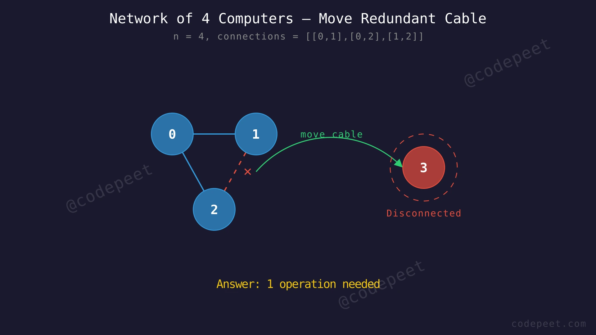
Input: n = 4, connections = [[0,1],[0,2],[1,2]]
Output: 1
Explanation: Computers 0, 1, and 2 are all connected to each other (they form a triangle). Computer 3 is completely isolated with no cables. The triangle has 3 cables but only needs 2 to keep all three computers connected — the cable between 1 and 2 is redundant (since 1 and 2 can still communicate through 0). We can remove the cable between 1 and 2 and use it to connect computer 3 to any of the other computers. This takes exactly 1 operation.
Example 2
Input: n = 6, connections = [[0,1],[0,2],[0,3],[1,2],[1,3]]
Output: 2
Explanation: Computers 0, 1, 2, and 3 are all connected. Computers 4 and 5 are each isolated. The group {0,1,2,3} has 5 cables but only needs 3 to stay connected — 2 cables are redundant. We need 2 extra cables to connect computer 4 and computer 5. We have exactly 2 redundant cables available, so we can connect everything with 2 operations.
Example 3
Input: n = 6, connections = [[0,1],[0,2],[0,3],[1,2]]
Output: -1
Explanation: We have 6 computers but only 4 cables. To connect 6 computers into a single network, we need at least 6 - 1 = 5 cables. Since 4 < 5, it is impossible to connect all computers no matter how we rearrange the cables. Return -1.
Constraints
- 1 ≤ n ≤ 10^5
- 1 ≤ connections.length ≤ min(n × (n - 1) / 2, 10^5)
- connections[i].length == 2
- 0 ≤ a_i, b_i < n
- a_i ≠ b_i
- There are no repeated connections.
- No two computers are connected by more than one cable.
Editorial
Brute Force
Intuition
Let us first observe a fundamental fact: to connect n computers into one network, we need at least n - 1 cables. This is because a connected network with no redundant cables forms a tree, and a tree with n nodes always has exactly n - 1 edges. If we have fewer cables than n - 1, it is impossible to connect everything — return -1 immediately.
Now, assuming we have enough cables, the question becomes: how many operations do we need?
Think of it like this: imagine the computers are people at a party, and cables are handshakes. Some people are already in groups (they can reach each other through chains of handshakes), while others are standing alone. To get everyone into one big group, we need to introduce each isolated group to the main group — that takes one "introduction" (operation) per extra group.
The most natural way to count these groups is to treat the network as a graph and find all connected components using Depth-First Search (DFS). We build an adjacency list from the connections, then launch DFS from every unvisited node. Each DFS discovers one complete connected component. After visiting all nodes, the number of connected components tells us the answer: we need (components - 1) operations to merge them all into one.
Step-by-Step Explanation
Let's trace through Example 1: n = 4, connections = [[0,1], [0,2], [1,2]]
Step 1: Check cable sufficiency. We need at least n - 1 = 3 cables. We have 3 cables. That is exactly enough, so we proceed.
Step 2: Build the adjacency list from connections:
- Node 0: neighbors [1, 2]
- Node 1: neighbors [0, 2]
- Node 2: neighbors [0, 1]
- Node 3: neighbors [] (no connections)
Initialize visited = [false, false, false, false] and components = 0.
Step 3: Node 0 is unvisited. Start DFS from node 0. Mark 0 as visited. Its neighbors are 1 and 2.
Step 4: DFS explores neighbor 1 from node 0. Mark 1 as visited. Traverse edge 0→1. Node 1's neighbors are 0 (already visited) and 2 (unvisited).
Step 5: DFS explores neighbor 2 from node 1. Mark 2 as visited. Traverse edge 1→2. Node 2's neighbors are 0 (already visited) and 1 (already visited). No unvisited neighbors remain.
Step 6: DFS backtracks. All nodes reachable from 0 have been visited: {0, 1, 2}. This forms connected component 1. Increment components to 1.
Step 7: Nodes 1 and 2 are already visited — skip them. Node 3 is unvisited. Start a new DFS from node 3. Mark 3 as visited. Node 3 has no neighbors, so DFS ends immediately. Node {3} forms connected component 2. Increment components to 2.
Step 8: All nodes visited. We found 2 connected components. The minimum operations needed = components - 1 = 2 - 1 = 1.
DFS Component Counting — Finding Connected Groups — Watch how DFS traversal discovers all nodes reachable from a starting node, identifying each connected component one at a time.
Algorithm
- If the number of connections is less than
n - 1, return-1(not enough cables to connect all computers). - Build an adjacency list from the
connectionsarray. - Initialize a
visitedarray of sizen(all false) and a countercomponents = 0. - For each node
ifrom0ton - 1:- If node
iis not visited:- Run DFS from node
i, marking all reachable nodes as visited. - Increment
componentsby 1.
- Run DFS from node
- If node
- Return
components - 1(the number of operations needed to merge all components into one).
Code
class Solution {
public:
    void dfs(int node, vector<vector<int>>& adj, vector<bool>& visited) {
        visited[node] = true;
        for (int neighbor : adj[node]) {
            if (!visited[neighbor]) {
                dfs(neighbor, adj, visited);
            }
        }
    }

    int makeConnected(int n, vector<vector<int>>& connections) {
        if ((int)connections.size() < n - 1) return -1;

        vector<vector<int>> adj(n);
        for (auto& conn : connections) {
            adj[conn[0]].push_back(conn[1]);
            adj[conn[1]].push_back(conn[0]);
        }

        vector<bool> visited(n, false);
        int components = 0;

        for (int i = 0; i < n; i++) {
            if (!visited[i]) {
                dfs(i, adj, visited);
                components++;
            }
        }

        return components - 1;
    }
};
class Solution:
def makeConnected(self, n: int, connections: List[List[int]]) -> int:
if len(connections) < n - 1:
return -1
adj = [[] for _ in range(n)]
for a, b in connections:
adj[a].append(b)
adj[b].append(a)
visited = [False] * n
components = 0
def dfs(node):
visited[node] = True
for neighbor in adj[node]:
if not visited[neighbor]:
dfs(neighbor)
for i in range(n):
if not visited[i]:
dfs(i)
components += 1
return components - 1class Solution {
public int makeConnected(int n, int[][] connections) {
if (connections.length < n - 1) return -1;
List<List<Integer>> adj = new ArrayList<>();
for (int i = 0; i < n; i++) {
adj.add(new ArrayList<>());
}
for (int[] conn : connections) {
adj.get(conn[0]).add(conn[1]);
adj.get(conn[1]).add(conn[0]);
}
boolean[] visited = new boolean[n];
int components = 0;
for (int i = 0; i < n; i++) {
if (!visited[i]) {
dfs(i, adj, visited);
components++;
}
}
return components - 1;
}
private void dfs(int node, List<List<Integer>> adj, boolean[] visited) {
visited[node] = true;
for (int neighbor : adj.get(node)) {
if (!visited[neighbor]) {
dfs(neighbor, adj, visited);
}
}
}
}Complexity Analysis
Time Complexity: O(V + E)
Where V = n (number of computers) and E = connections.length (number of cables). Building the adjacency list takes O(E) time since we iterate over all connections once. The DFS traversal visits each node exactly once and explores each edge exactly twice (once from each endpoint), giving O(V + E) total. Combined: O(V + E).
Space Complexity: O(V + E)
The adjacency list stores each edge twice (once for each endpoint), requiring O(V + E) space. The visited array takes O(V) space. The DFS recursion stack can go as deep as O(V) in the worst case (a chain-shaped graph). Total: O(V + E).
Why This Approach Is Not Efficient
The DFS approach correctly solves the problem in O(V + E) time, which is already efficient. However, it has several practical drawbacks that a more elegant approach can avoid:
1. Space Overhead of the Adjacency List: DFS requires building a full adjacency list from all connections before any traversal can begin. This takes O(V + E) space. For a network with 100,000 computers and nearly as many cables, this means allocating significant memory just to represent the graph structure. If we could process edges directly without building the full graph, we would save space.
2. Recursion Stack Risk: DFS uses recursion, and the call stack depth can reach O(V) in the worst case (imagine 100,000 computers linked in a single chain). In languages like Python with default recursion limits (~1000), this causes a stack overflow. While iterative DFS can solve this, it adds implementation complexity.
3. No Natural Redundancy Detection: The DFS approach counts components but does not naturally identify which specific cables are redundant. It relies on the mathematical fact that if we have ≥ n-1 cables, we definitely have enough redundant ones. A different data structure could track redundancy as a natural byproduct.
Key Insight: The Union-Find (Disjoint Set Union) data structure can process edges one at a time, tracking both the number of components and redundant cables simultaneously. It needs only O(V) space (no adjacency list), avoids recursion entirely, and is specifically designed for connectivity problems.
Optimal Approach - Union-Find (Disjoint Set Union)
Intuition
Union-Find is a data structure built specifically for answering connectivity questions: "Are these two elements in the same group?" and "Merge these two groups together." It is a perfect fit for this problem.
The idea is simple. Initially, every computer is its own isolated group (its own connected component). We maintain a parent array where parent[i] tells us which group node i belongs to. At first, parent[i] = i — every node is its own parent, meaning it is alone.
Then we process each cable (edge) one at a time:
- For the cable connecting computers
aandb, we find the root (ultimate parent) of each. - If they have the same root, they are already in the same group. This cable is redundant — it creates a cycle and does not add connectivity.
- If they have different roots, they are in separate groups. We union them by making one root point to the other, merging the two groups into one. This reduces our total component count by 1.
After processing all cables, we know:
- How many connected components remain (started at
n, decreased by 1 for each successful union). - How many redundant cables exist (each same-root edge).
The answer is simply components - 1: the number of additional connections needed to link all components into one network. If we do not have enough total cables (fewer than n - 1), return -1.
The beauty of Union-Find with path compression is that the find operation is nearly O(1) amortized, making the entire algorithm extremely fast in practice.
Step-by-Step Explanation
Let's trace through Example 1: n = 4, connections = [[0,1], [0,2], [1,2]]
Step 1: Check cable sufficiency. Need n - 1 = 3 cables. Have 3 cables. Sufficient, proceed.
Step 2: Initialize the parent array: parent = [0, 1, 2, 3]. Each computer is its own parent — 4 separate components. Set components = 4 and redundant = 0.
Step 3: Process edge [0, 1].
- find(0) = 0 (parent[0] = 0, it is its own root).
- find(1) = 1 (parent[1] = 1, it is its own root).
- Different roots (0 ≠ 1) → union them. Set parent[0] = 1.
- Parent array: [1, 1, 2, 3]. Components = 3.
Step 4: Process edge [0, 2].
- find(0): parent[0] = 1, parent[1] = 1 (root). Root of 0 is 1.
- find(2) = 2 (parent[2] = 2, it is its own root).
- Different roots (1 ≠ 2) → union them. Set parent[1] = 2.
- Parent array: [1, 2, 2, 3]. Components = 2.
Step 5: Process edge [1, 2].
- find(1): parent[1] = 2, parent[2] = 2 (root). Root of 1 is 2.
- find(2) = 2 (parent[2] = 2, root).
- Same root (both 2)! This cable is redundant — nodes 1 and 2 are already connected. Redundant = 1.
Step 6: All edges processed. Components = 2 (group {0,1,2} and group {3}). Need components - 1 = 1 cable to connect them. Have 1 redundant cable ≥ 1 needed. Answer = 1.
Union-Find — Tracking Parent Array and Component Merges — Watch how the parent array evolves as we process each edge. Each successful union merges two components; same-root edges reveal redundant cables.
Algorithm
- If the number of connections is less than
n - 1, return-1(impossible to connect all computers). - Initialize a
parentarray of sizenwhereparent[i] = i. - Set
components = n(each node starts as its own component). - For each connection
[a, b]:- Find the root of
ausing thefindfunction (with path compression). - Find the root of
busing thefindfunction. - If roots are different: union them by setting
parent[rootA] = rootB, then decrementcomponents. - If roots are the same: this edge is redundant (skip).
- Find the root of
- Return
components - 1.
Code
class Solution {
    vector<int> parent;

    int find(int x) {
        if (parent[x] != x) {
            parent[x] = find(parent[x]);
        }
        return parent[x];
    }

public:
    int makeConnected(int n, vector<vector<int>>& connections) {
        if ((int)connections.size() < n - 1) return -1;

        parent.resize(n);
        iota(parent.begin(), parent.end(), 0);

        int components = n;
        for (auto& conn : connections) {
            int rootA = find(conn[0]);
            int rootB = find(conn[1]);
            if (rootA != rootB) {
                parent[rootA] = rootB;
                components--;
            }
        }

        return components - 1;
    }
};
class Solution:
def makeConnected(self, n: int, connections: List[List[int]]) -> int:
if len(connections) < n - 1:
return -1
parent = list(range(n))
def find(x):
if parent[x] != x:
parent[x] = find(parent[x])
return parent[x]
components = n
for a, b in connections:
root_a, root_b = find(a), find(b)
if root_a != root_b:
parent[root_a] = root_b
components -= 1
return components - 1class Solution {
int[] parent;
int find(int x) {
if (parent[x] != x) {
parent[x] = find(parent[x]);
}
return parent[x];
}
public int makeConnected(int n, int[][] connections) {
if (connections.length < n - 1) return -1;
parent = new int[n];
for (int i = 0; i < n; i++) parent[i] = i;
int components = n;
for (int[] conn : connections) {
int rootA = find(conn[0]);
int rootB = find(conn[1]);
if (rootA != rootB) {
parent[rootA] = rootB;
components--;
}
}
return components - 1;
}
}Complexity Analysis
Time Complexity: O(E × α(V)) ≈ O(E)
Where E = connections.length and V = n. For each of the E edges, we perform two find operations and potentially one union. With path compression, each find call runs in O(α(V)) amortized time, where α is the inverse Ackermann function — a function that grows so slowly it is effectively constant (≤ 4) for any practical input size. Thus the total time is O(E × α(V)), which is practically O(E).
Space Complexity: O(V)
We only need the parent array of size V. Unlike the DFS approach, we do not build an adjacency list (saving O(E) space) and do not use a recursion stack. The total space is simply O(V), which is a meaningful improvement over the DFS approach's O(V + E) space, especially for dense graphs where E can be much larger than V.