uber
Introduction
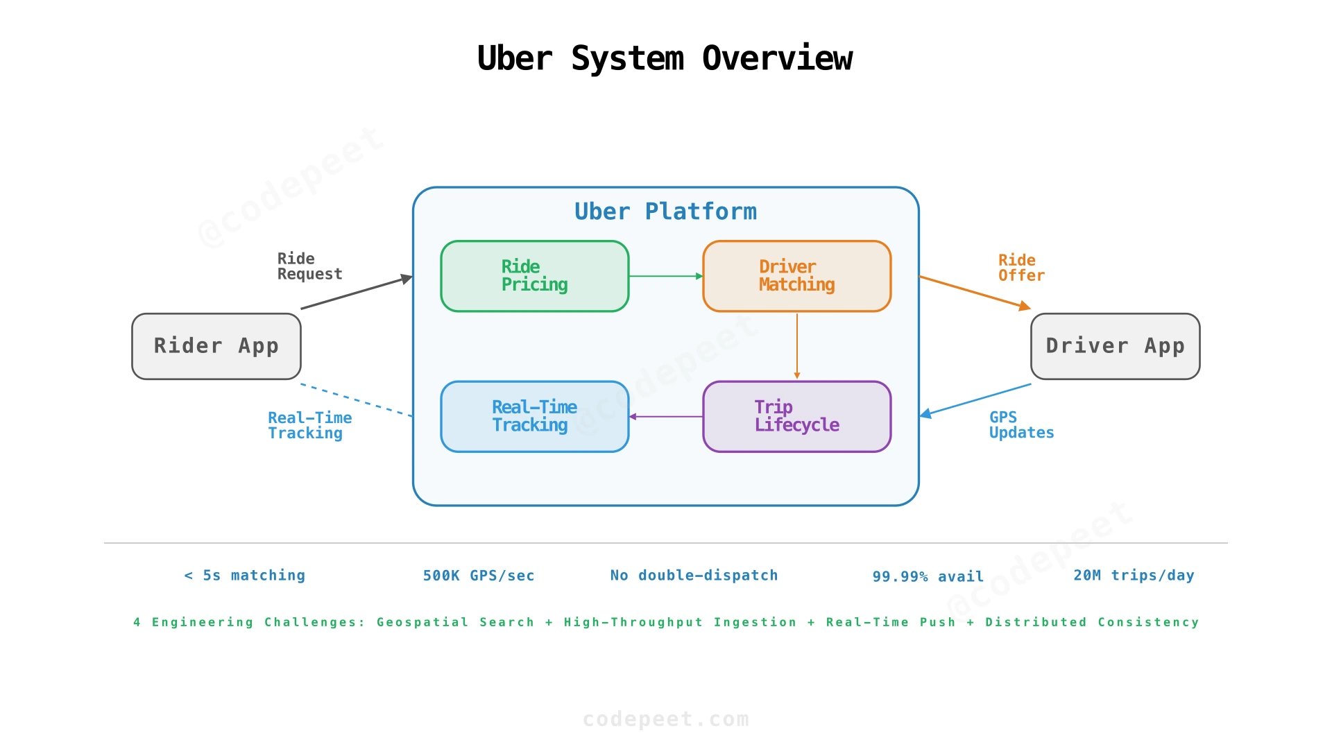
Uber is a ride-hailing service where a rider requests a ride, the system estimates the fare, finds nearby available drivers, and matches one to the rider. During the trip, the system tracks the driver's real-time location and streams updates to the rider's map. The trip moves through a lifecycle of states — searching, matched, in progress, completed — with each transition triggering side effects like notifications, fare metering, and payment.
What makes Uber architecturally fascinating is that it sits at the intersection of four distinct engineering challenges, each demanding a different class of infrastructure:
- Geospatial Search — Finding nearby drivers among millions of moving objects. Standard B-tree indexes on latitude/longitude don't work; you need spatial data structures (geohash, quadtree, H3) that group nearby points together.
- High-Throughput Ingestion — Two million online drivers sending GPS coordinates every 4 seconds produces ~500,000 writes/sec at peak. No relational database handles this on a single table with durable commits. Separating the hot path (in-memory for real-time matching) from the cold path (async persistence for history) is essential.
- Real-Time Communication — The rider must see the driver's car icon move on their map in near real-time. This requires persistent WebSocket connections, a connection registry to route messages across server instances, and graceful handling of mobile network disconnections.
- Distributed Consistency — A driver must never be assigned to two riders simultaneously (double-dispatch). Trip state transitions must be atomic with reliable side effects. This demands optimistic concurrency control and the transactional outbox pattern.
The system handles ~20 million trips per day across 50 million daily active riders and 5 million registered drivers. At peak, 2 million drivers are online simultaneously, generating half a million location updates per second. The architecture must deliver sub-5-second ride matching while maintaining strict consistency on driver assignment.
Functional Requirements
We extract verbs from the problem statement to identify core operations:
- "estimates the fare" and "calculates the route" → COMPUTE operation (Ride Pricing)
- "finds nearby drivers" and "matches one to the rider" → SEARCH + ASSIGN operation (Find and Match a Driver)
- "tracks the driver's location" and "streams updates" → INGEST + PUSH operation (Real-Time Tracking)
- "moves through a lifecycle of states" with side effects → STATE MACHINE operation (Trip Lifecycle)
Each verb maps to a functional requirement. Each requirement builds on the previous, progressively adding components to the architecture.
-
Ride Pricing — Rider enters a pickup location and destination. The system returns an estimated fare and ETA before the rider confirms the request.
-
Find and Match a Driver — After the rider confirms, the system finds nearby available drivers, ranks them, and assigns one through an offer/accept flow.
-
Real-Time Driver Tracking — Online drivers continuously report GPS coordinates. During an active trip, the rider sees the driver's live position on a map in near real-time.
-
Trip Lifecycle Management — The system manages the full lifecycle of a trip through well-defined states, with each transition triggering appropriate side effects (notifications, metering, payment).
Out of Scope
- Payment processing and billing integration (assume a separate payment service)
- Driver onboarding, background checks, and document verification
- Ride scheduling (booking for a future time)
- Shared rides / carpooling (UberPool-style splitting)
- Multi-stop trips
- In-app messaging or calling between rider and driver
- Driver earnings, tips, and incentive programs
Non-Functional Requirements
We extract adjectives and descriptive phrases from the problem statement to identify quality constraints:
- "real-time" location tracking → Low-latency updates; the rider must see the driver's position move smoothly on the map
- "millions of drivers" sending GPS "every few seconds" → High write throughput on location ingestion (~500K writes/sec at peak)
- "sub-second" geospatial searches → Fast nearby-driver lookup via spatial index, separate from end-to-end matching which includes the offer/accept flow
- "unique" driver assignment (no double-dispatch) → Strict consistency on driver assignment; under partitions, reject or queue rather than risk double-assignment
- "persistent" and "durable" trip records → Trip data and fare records must survive failures; state transitions must be atomic
- "consistent" trip lifecycle → Side effects triggered reliably (at-least-once) with idempotency/deduplication for effectively-once outcomes
| NFR | Target | Reasoning |
|---|---|---|
| Low Latency | Sub-second geospatial lookup; end-to-end ride matching within 5 seconds | Riders expect near-instant driver assignment |
| High Throughput | ~500K location writes/sec at peak; 20M trips/day | 2M online drivers × 1 update every 4 seconds |
| Strong Consistency | No double-dispatch; atomic trip state transitions | A driver must never be assigned to two riders simultaneously |
| High Availability | 99.99% for ride requests and tracking | Ride-hailing is a real-time service; downtime means lost revenue and stranded riders |
| Durability | Trip records survive any single-node failure | Legal, financial, and dispute resolution requirements |
Key insight: These NFRs are in tension. Strong consistency on driver assignment conflicts with high availability under network partitions (CAP theorem). The system resolves this by choosing consistency over availability for the assignment operation specifically — it's better to fail a match attempt and retry with the next driver than to double-assign. All other operations (location ingestion, tracking, fare estimation) favor availability.
Resource Estimation
Scale Assumptions
| Parameter | Value |
|---|---|
| Daily active riders | ~50 million |
| Registered drivers | ~5 million |
| Peak online drivers | ~2 million |
| Trips per day | ~20 million |
| Driver location update interval | ~4 seconds (average during peak) |
Throughput
Location writes (peak):
Ride requests (average):
WebSocket connections (peak):
Storage
Location data (per day):
Each location update ≈ 100 bytes (driver_id, lat, lng, heading, speed, timestamp, trip_id).
With 90-day retention for detailed location history (aggregated thereafter):
Trip records:
Each trip record ≈ 1 KB (IDs, coordinates, fares, timestamps, status).
Bandwidth
Inbound (GPS ingestion):
Outbound (rider tracking):
Assume ~2M active trips at peak, each rider receiving updates every 4 seconds (~200 bytes with driver info + coordinates):
API Design
We derive API endpoints directly from the functional requirements (verbs identified above). Most real-time communication happens over WebSocket, but the API defines the REST surface for ride operations.
REST Endpoints
# ── Fare Estimate ─────────────────────────────────────────────
GET /rides/estimate?pickup_lat={lat}&pickup_lng={lng}&dest_lat={lat}&dest_lng={lng}
→ 200 OK
{
  "estimated_fare": { "amount": 24.50, "currency": "USD" },
  "estimated_duration_min": 23,
  "estimated_distance_km": 12.4,
  "surge_multiplier": 1.0
}

# ── Request a Ride ────────────────────────────────────────────
POST /rides
{
  "pickup": { "lat": 37.7749, "lng": -122.4194 },
  "destination": { "lat": 37.3382, "lng": -121.8863 },
  "vehicle_type": "standard"
}
→ 201 Created
{
  "ride_id": "ride_abc123",
  "status": "SEARCHING"
}

# ── Get Ride Status ───────────────────────────────────────────
GET /rides/{id}
→ 200 OK
{
  "ride_id": "ride_abc123",
  "status": "MATCHED",
  "driver": {
    "id": "d456", "name": "Maria",
    "vehicle": "Silver Toyota Camry",
    "license_plate": "ABC1234"
  },
  "pickup_eta_min": 3,
  "estimated_fare": { "amount": 24.50, "currency": "USD" }
}

# ── Cancel a Ride ─────────────────────────────────────────────
POST /rides/{id}/cancel
→ 200 OK  { "status": "CANCELLED", "cancellation_fee": 0 }

# ── Driver Accepts/Declines Offer ─────────────────────────────
POST /rides/{id}/offer/accept
→ 200 OK  { "status": "MATCHED", "pickup": {...}, "rider": {...} }

POST /rides/{id}/offer/decline
→ 200 OK  { "status": "declined" }

# ── Update Driver Location (HTTP fallback) ────────────────────
PUT /drivers/{id}/location
{ "lat": 37.7751, "lng": -122.4180, "heading": 45,
  "speed_kmh": 30, "timestamp": "2024-01-15T10:30:00Z" }
→ 200 OK  { "status": "ok" }

# ── Rate a Ride ───────────────────────────────────────────────
POST /rides/{id}/rating
{ "stars": 5, "comment": "Great ride" }
→ 200 OK  { "status": "ok" }
WebSocket Protocol
Both rider and driver apps maintain a persistent WebSocket connection to the Connection Service. The WebSocket carries all real-time communication:
| Direction | Message Type | Payload |
|---|---|---|
| Driver → Server | location_update | {lat, lng, heading, speed, timestamp} |
| Server → Driver | ride_offer | {ride_id, pickup, destination, fare} |
| Server → Driver | ride_cancelled | {ride_id, reason} |
| Server → Rider | driver_location | {lat, lng, heading, eta_min} |
| Server → Rider | ride_matched | {driver_id, name, vehicle, eta} |
| Server → Rider | trip_state_change | {ride_id, new_state, metadata} |
Data Model
The data model is derived from extracting nouns in the problem statement. Three core entities drive the architecture:
Trip — Core entity tracking a ride from request to completion. Each trip moves through states (SEARCHING, MATCHED, ARRIVED, IN_PROGRESS, COMPLETED, CANCELLED).
| Field | Type | Description |
|---|---|---|
trip_id | string | Primary key |
rider_id | string | FK to the rider |
driver_id | string | FK to assigned driver (null during SEARCHING) |
status | enum | Current state in the trip state machine |
pickup_lat/lng | float | Pickup coordinates |
dest_lat/lng | float | Destination coordinates |
estimated_fare | decimal | Fare estimate shown before confirmation |
actual_fare | decimal | Final fare after completion |
created_at | timestamp | When the ride was requested |
completed_at | timestamp | When the trip ended |
DriverLocation — Real-time GPS position. Updated every ~4 seconds. Stored in-memory for matching, persisted asynchronously for history.
| Field | Type | Description |
|---|---|---|
driver_id | string | FK to the driver |
trip_id | string | Nullable; set during active trip |
lat/lng | float | Current GPS coordinates |
geohash | string | Precomputed for spatial indexing |
heading | int | Direction of travel (0-360°) |
speed_kmh | float | Current speed |
timestamp | timestamp | When recorded by driver's device |
Driver — Profile and availability. The version field supports optimistic concurrency for double-dispatch prevention.
| Field | Type | Description |
|---|---|---|
driver_id | string | Primary key |
name | string | Display name shown to riders |
vehicle_info | string | Make, model, color, license plate |
status | enum | available, offered, en_route_to_pickup, on_trip, offline |
current_trip_id | string | Nullable; active trip assignment |
version | int | Optimistic lock version for double-dispatch prevention |
Relationships: Trip ↔ Driver is many-to-one (a driver has many trips over time; each trip has at most one driver). Trip ↔ DriverLocation is one-to-many (a trip's route is reconstructed from location snapshots with matching trip_id).
High-Level Design
We build the architecture progressively, one functional requirement at a time. Each step introduces new components that address specific NFR challenges. The architecture diagram grows from 2 services to the full system across 4 steps.
Step 1: Ride Pricing — Route-Based Fare Estimation
The Starting Architecture
A rider opens the app, types "SFO Airport" as the destination, and sees "$24.50, ~23 min." This estimate appears before they commit to the ride. Let's build the pricing flow.
The Problem
Fare depends on the actual driving route, not the straight-line distance between two points. A 10km straight line might be 15km of road with turns, highway ramps, and one-way streets. Straight-line pricing would consistently undercharge for complex routes and overcharge for highway trips.
Route Calculation via Routing Service
The Ride Service sends the pickup and destination coordinates to a Routing Service. The Routing Service models the road network as a weighted graph: intersections are nodes, road segments are edges, weights are expected travel times. A shortest-path algorithm (Dijkstra or A* variant) finds the fastest route and returns the total distance and estimated duration.
# Fare calculation formula
fare = base_fare + (distance_km × per_km_rate) + (duration_min × per_min_rate)

# With surge pricing (if active in the pickup zone)
final_fare = fare × surge_multiplier
The rider sees the estimate and taps "Confirm." The system creates a ride request with status SEARCHING and begins the matching process.
The architecture at this stage is straightforward: the Rider App sends a fare estimate request through the API Gateway to the Ride Service. The Ride Service calls the Routing Service for route distance and duration, computes the fare, and stores the trip record in the Trip DB. Two services, one database.
✅ NFR addressed: Basic fare estimation working
❌ Still missing: No way to find nearby drivers — a
SELECT *scanning all 2M online drivers is unacceptable. No real-time tracking. No trip lifecycle management.
Step 2: Geospatial Matching — Finding and Assigning Drivers
Adding Spatial Search + Driver Matching
The rider confirmed the ride. The system needs to answer: "Which available drivers are near this rider?" and assign the best one.
The Problem
The naive approach queries the driver database directly:
SELECT * FROM drivers
WHERE status = 'available'
  AND distance(lat, lng, 37.77, -122.41) < 3000
ORDER BY distance
LIMIT 5;
With 2 million online drivers and no spatial index, this query calculates distance for every row. Standard B-tree indexes on latitude or longitude alone don't help — they narrow one dimension but still scan thousands of candidates in the other. At 1,000 ride requests per second during peak, each full-scan query holds a connection for hundreds of milliseconds, exhausting the connection pool.
Geospatial Index for Nearby Search
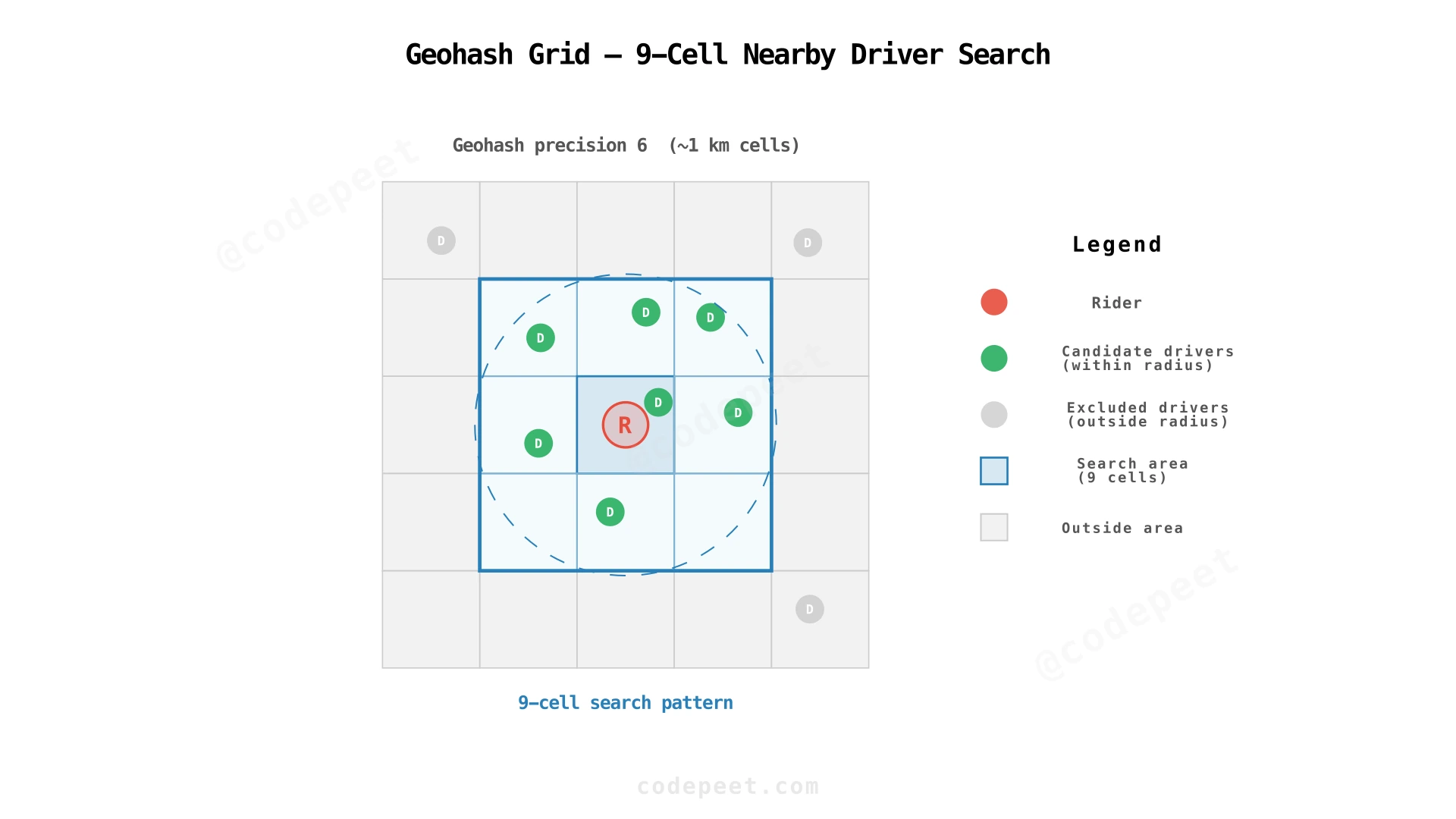
Instead of scanning all drivers, organize driver locations in a geospatial index that groups nearby drivers together. We use geohash-based spatial indexing: encode each driver's coordinates into a string where nearby locations share a common prefix.
When a rider requests a ride:
- Compute the rider's geohash at the search precision (e.g., precision 6, roughly ~1km-scale cells)
- Query the rider's cell and all 8 neighboring cells — the 9-cell search pattern handles drivers near cell boundaries
- Filter to
availabledrivers only, compute actual distances, remove any beyond the maximum search radius - Rank remaining candidates by distance from the rider's pickup point
If the initial search returns too few candidates (common in suburban areas), expand to a coarser geohash precision (~5km × 5km cells). Keep expanding until enough candidates are found or the maximum radius is reached.
Geospatial Indexing Options
Geohash Grid — Encode lat/lng into a string. Nearby locations share a prefix. Store drivers in a set keyed by their geohash cell; look up the cell and its 8 neighbors. Updates are simple: when a driver moves to a new cell, remove from the old set and add to the new one. Limitation: fixed cell sizes don't adapt to density. Manhattan might have 200 drivers per cell; rural areas have zero.
QuadTree — Recursively divide space into four quadrants. Dense areas subdivide further; sparse areas stay coarse. Adapts to driver density naturally. Limitation: in-memory data structure that doesn't map to key-value stores easily. Distributing across servers requires custom sharding.
R-Tree — Groups nearby objects into bounding rectangles in a balanced tree. Built into spatial databases (PostGIS). Efficient for read-heavy workloads. Limitation: insertion/deletion requires rectangle rebalancing — write amplification becomes costly at 500K updates/sec.
H3 Hexagonal Grid — H3 divides Earth into hexagonal cells at 16 resolution levels. Most cells have 6 neighbors at near-uniform adjacency distances — no corner-distance problem of rectangular grids. Limitation: requires a library for icosahedral projection math.
Recommendation: Use geohash as the default in a system design interview — it's the simplest to explain. If asked about production improvements, mention H3 for uniform neighbor distances and multi-resolution support.
Send Offer and Match
With a ranked list of nearby available drivers, the Matching Service sends a ride offer to the nearest candidate via their WebSocket connection: "New ride request, pickup at X, destination Y. Accept?"
The driver has a timeout window (e.g., 15 seconds) to respond:
- Accept: The ride transitions to
MATCHED. The rider is notified with driver details and ETA. - Decline or timeout: The system tries the next candidate on the list.
If all candidates decline, expand the search radius and try again. If no driver is found after all retries, notify the rider: "No drivers available."
⚠️ A critical correctness problem exists here: what if two ride requests simultaneously try to assign the same driver? This double-dispatch problem is covered in the Deep Dive section.
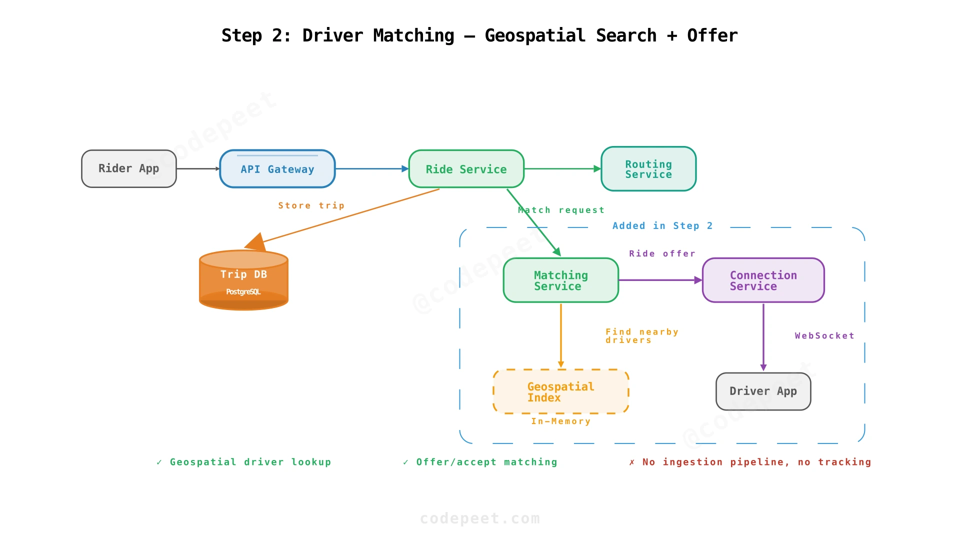
The architecture now adds three components. The Matching Service receives ride requests and queries the Geospatial Index (in-memory) for nearby available drivers. It sends ride offers to drivers through the Connection Service, which maintains WebSocket connections to Driver Apps.
✅ NFRs addressed: Sub-second geospatial lookup (geohash index), driver matching via offer/accept flow
❌ Still missing: No pipeline for ingesting 500K GPS updates/sec — who populates the geospatial index? No real-time rider tracking. No double-dispatch prevention. No trip lifecycle management.
Step 3: Real-Time Location Pipeline — High-Throughput GPS Ingestion
Adding the Location Ingestion Pipeline + Real-Time Tracking
The ride is matched. The rider is watching their phone, waiting for the driver's car icon to appear and move toward them. This requires two things: a pipeline to ingest driver GPS updates at massive scale, and a way to push those updates to the rider's device in real-time.
The Problem
Two million online drivers send GPS coordinates every 4 seconds. That's roughly 500,000 writes per second at peak — potentially bursty without client-side jitter. And during an active trip, each location update must reach the rider's phone within seconds.
WebSocket Connections
Both rider and driver apps maintain a persistent WebSocket connection to a Connection Service. WebSocket provides a bidirectional channel: the driver sends location updates upstream, receives ride offers downstream. The rider sends ride requests upstream, receives tracking updates downstream.
Real-Time Communication Options
Short Polling — Client sends an HTTP request every N seconds. Simple, works through all proxies. But at 2M drivers polling every 2 seconds, that's 1M requests/sec of pure overhead — most responses empty. Latency equals the polling interval.
Server-Sent Events (SSE) — Server pushes events over a long-lived HTTP connection. No polling overhead, low latency. But SSE is one-way (server → client). Drivers still need a separate upstream path for sending locations.
WebSocket (Recommended) — Persistent bidirectional connection. Both sides send messages at any time. One connection handles both upload (location) and download (offers, tracking). Lower per-message overhead than full HTTP headers.
Tradeoff: connections are stateful. The server tracks which connection belongs to which user. A connection registry is needed to locate and deliver server-initiated pushes to the correct Connection Service instance.
Why WebSocket: Ride-hailing needs bidirectional, low-latency communication. The driver sends GPS upstream and receives offers downstream. WebSocket handles both over a single persistent connection.
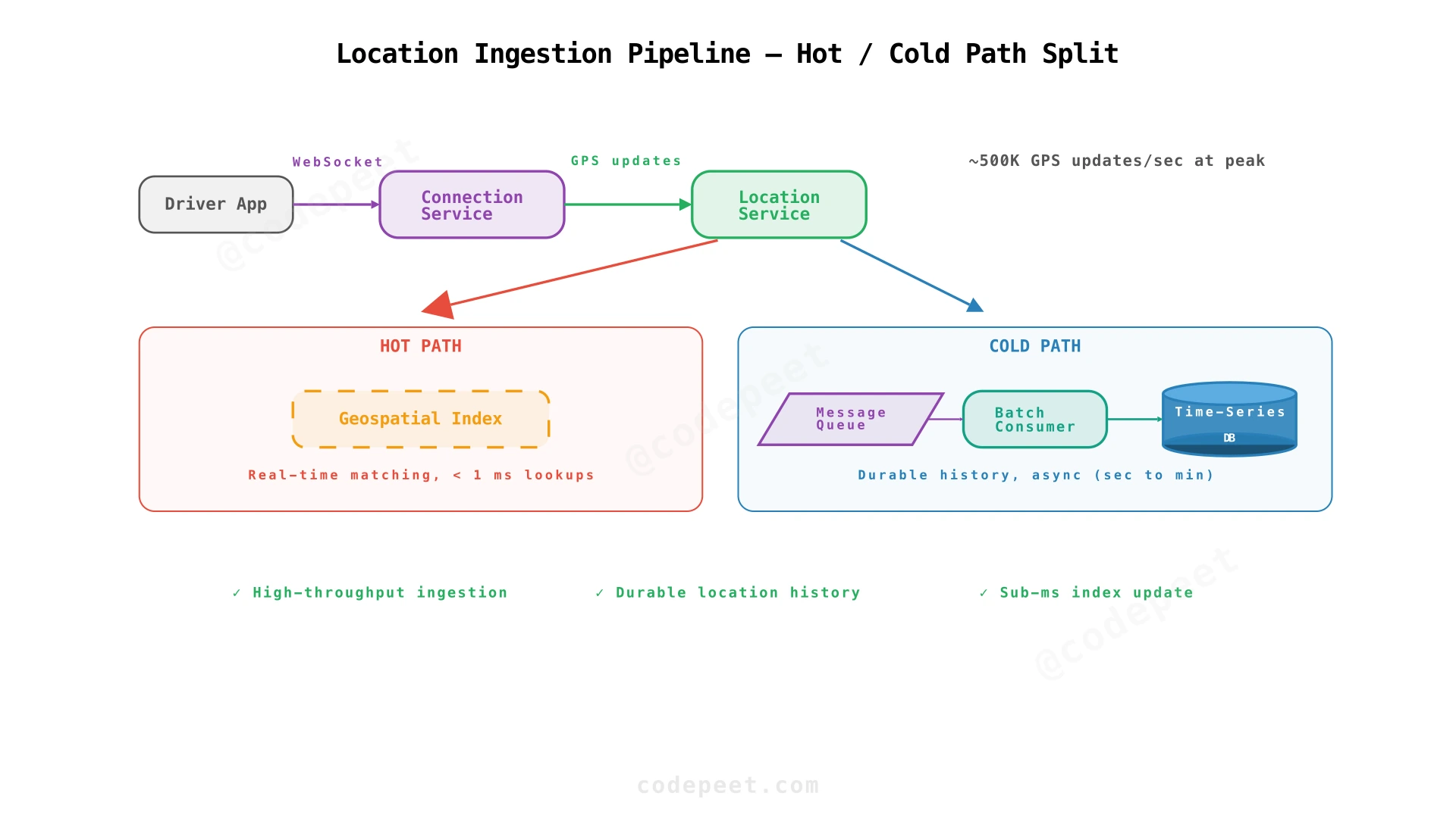
Location Ingestion Pipeline
Every 4 seconds, each online driver's app sends a location update over their WebSocket connection: {driver_id, lat, lng, timestamp, heading, speed}. The Location Service receives these updates and splits them into two paths:
-
Hot Path — Update the in-memory Geospatial Index. Compute the driver's geohash. Store the driver's position under that geohash key. If the driver moved to a new cell, remove from the old cell and add to the new one. This is what the Matching Service reads from. Typically low-millisecond latency per operation.
-
Cold Path — Persist location updates asynchronously for durability (trip history, analytics, dispute resolution). A message queue buffers updates; a consumer writes them to a time-series database in batches. No strict sub-second requirement, but keep end-to-end lag bounded (seconds to minutes).
The hot path handles the throughput challenge. The cold path handles the durability requirement. Neither needs to do both.
Location Relay to Rider
When a driver's location update arrives and the driver is on an active trip, the Location Service forwards it to the rider. But the rider is connected to a different Connection Service instance. How does the Location Service know which instance?
A connection registry (an in-memory key-value store) maps user_id → connection_service_instance. When a client connects, the Connection Service registers the mapping with a short TTL and periodic heartbeats. Any backend service that needs to push a message looks up the registry and routes to the correct instance.
Full flow: Driver App → Connection Service A → Location Service → [update index] → look up rider's connection → Connection Service B → rider's WebSocket → rider app renders position on map.
The rider sees the driver's position update every few seconds. The client interpolates between updates to produce smooth map animation.
Handling Disconnections
Mobile networks are unreliable. When a rider's WebSocket drops (tunnel, elevator), the system buffers recent events for each active trip. On reconnection, the client sends its last-seen event timestamp, and the server replays anything newer.
The architecture now adds four components. The Location Service receives GPS updates and splits them: the hot path updates the in-memory Geospatial Index, the cold path sends updates through a Message Queue to a Time-Series DB. The Connection Registry maps users to their Connection Service instance for cross-instance message routing.
✅ NFRs addressed: 500K writes/sec via in-memory index (high throughput), real-time driver-to-rider tracking via WebSocket (low latency), durable location history via async cold path
❌ Still missing: Trip state transitions are ad-hoc — no formal state machine. Side effects (notifications, payment) aren't reliably triggered. Double-dispatch still possible if two matching requests race on the same driver.
Step 4: Complete Architecture — Trip Lifecycle with Consistency Guarantees
Adding the Trip State Machine + Double-Dispatch Prevention
So far we've covered how the rider gets a fare estimate, how the system finds and matches a driver, and how location updates flow in real-time. Now we need to manage what happens after matching: the driver drives to the pickup, picks up the rider, drives to the destination, and completes the trip. Each phase has different rules and different data flowing to both parties.
The Problem
A ride involves many state changes: searching → matched → driver arrived → trip in progress → completed. Each transition triggers different side effects. When the driver is matched, the rider needs a notification. When the trip starts, fare metering begins. When it completes, payment is triggered. Without a formal state machine, these transitions become ad-hoc and error-prone — a missed notification, a fare that never starts metering, a payment that fires twice.
Trip State Machine
A trip moves through these states:
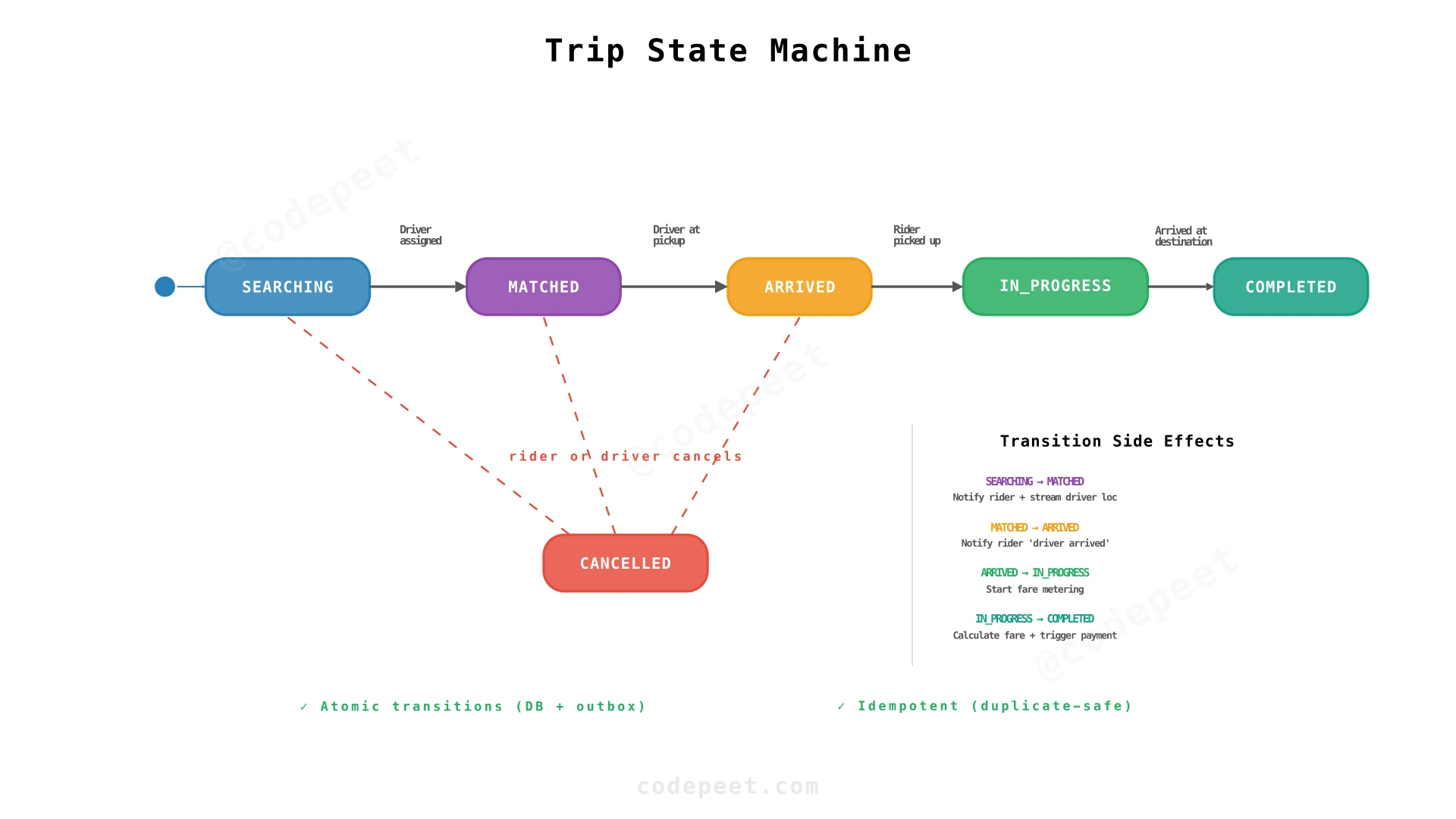
- SEARCHING — Rider requested, system is finding a driver
- MATCHED — Driver assigned, en route to pickup location
- ARRIVED — Driver reached the pickup, waiting for rider
- IN_PROGRESS — Rider picked up, driving to destination
- COMPLETED — Arrived at destination, fare calculated
- CANCELLED — Cancelled by rider or driver (rules depend on current state)
Each transition is performed atomically in a single database transaction (conditional state update + outbox insert). The Trip Service validates that the transition is legal (e.g., you can't jump from SEARCHING to IN_PROGRESS) and updates the record.
Reliable Event Publishing via Outbox Pattern
To reliably publish events after each transition, the service writes the event to an outbox table in the same database transaction as the state change. A separate process reads the outbox and publishes domain events (trip.matched, trip.started, trip.completed) to a message queue for downstream consumers. This avoids the dual-write problem where the DB update succeeds but the event publish fails.
Transition Side Effects
| Transition | Side Effects |
|---|---|
| SEARCHING → MATCHED | Notify rider with driver details; start streaming driver's location; notify driver with pickup navigation |
| MATCHED → ARRIVED | Notify rider "Your driver has arrived"; start wait timer (5 min) |
| ARRIVED → IN_PROGRESS | Start fare metering (distance + time tracking); switch navigation to destination |
| IN_PROGRESS → COMPLETED | Calculate final fare; trigger payment; prompt ratings |
| Any → CANCELLED | Rules depend on state (free during SEARCHING, fee after MATCHED) |
Idempotent Transitions
Network issues can cause duplicate transition requests. If the driver's app sends "arrived at pickup" twice due to a retry, the Trip Service handles this gracefully. Each transition checks the current state before applying. If the trip is already ARRIVED, a duplicate "arrived" request is a no-op. Side effects also need deduplication via idempotency keys or unique constraints in the outbox.
Double-Dispatch Prevention
When the Matching Service tries to assign a driver, it performs a conditional update with optimistic concurrency:
UPDATE driver
SET status = 'offered',
    current_trip_id = 'R1',
    version = 43
WHERE id = 'A'
  AND status = 'available'
  AND version = 42;
-- If 1 row affected → reservation succeeded
-- If 0 rows affected → another request beat us; try next driver
The version field prevents a subtle edge case: a driver going available → offered → available → offered in quick succession where a stale retry from the first cycle lands during the second. Without the version check, the retry would succeed because status is available again.
Fare Estimation vs Actual Fare
The estimated fare (from Step 1) uses expected route distance and time. The actual fare is calculated from metered distance and time after the trip completes. If the actual fare differs significantly (e.g., driver took a much longer route), the system can flag it for review or cap the fare at the estimate.
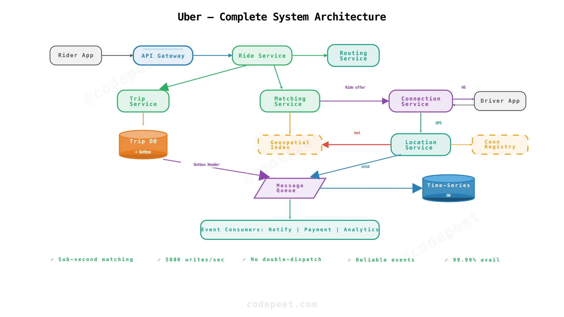
The final architecture adds three components. The Trip Service manages the state machine, writing each transition atomically to the Trip DB + Outbox. An outbox reader publishes domain events to the Message Queue. Event Consumers subscribe and handle side effects: notifications, payment, and analytics.
NFR Scorecard
| NFR | Target | How It's Met |
|---|---|---|
| Low Latency | Sub-second geospatial lookup; <5s ride matching | In-memory geohash index (<1ms lookups); WebSocket for instant push; connection registry for cross-instance routing |
| High Throughput | 500K location writes/sec | Hot/cold path separation; in-memory geospatial index for writes; async batch persistence to time-series DB; sharded by geographic region |
| Strong Consistency | No double-dispatch; atomic state transitions | Optimistic concurrency control (version-based conditional UPDATE) on driver assignment; Trip Service validates state machine transitions atomically |
| High Availability | 99.99% for ride requests and tracking | Stateless services behind load balancers; connection registry with replica promotion; geospatial index rebuilds from driver re-reports or MQ replay within seconds |
| Durability | Trip records survive any single-node failure | Trip DB with replication; outbox pattern ensures events are never lost; cold path persists location history to time-series DB |
| Reliability | Side effects trigger exactly-once | Outbox pattern avoids dual-write problem; idempotent transitions with deduplication keys; at-least-once delivery with idempotent consumers |
Deep Dives
How do you handle 500,000 driver location updates per second?
Location Update Scale
Two million online drivers, each sending GPS coordinates every 4 seconds. That's roughly 500,000 writes per second at peak, with spikes during rush hour. A relational database doing 500K durable random writes per second on a single table would struggle — WAL/fsync overhead, index maintenance, and transaction coordination make this impractical.
Separating Hot and Cold Paths
The geospatial index for real-time matching doesn't need durability. If it crashes, connected drivers will send new updates within a few seconds — though mobile network conditions and reconnection delays mean full recovery may take longer. Replication or replay from a recent snapshot helps close this gap.
- Hot path: Driver → Location Service → in-memory geospatial index. Typically low-millisecond writes. This is what matching queries read from.
- Cold path: Location Service → message queue → batch consumer → time-series database. Writes in batches of thousands. No strict sub-second requirement, but keep end-to-end lag bounded for consumers like dispute resolution.
Sharding the Geospatial Index
Even in-memory, a single node handling 500K writes per second may hit CPU limits. Shard the index by geographic region: North America, Europe, Asia, etc. Each shard handles drivers in its region only.
Within a region, further partition by city or metro area. The sharding key is the driver's coarse geohash prefix (first 2-3 characters). Most proximity queries stay local to one shard. For riders near a shard boundary, fan out the query to the adjacent shard — handled by checking which shard owns each of the 9 neighboring cells.
Adaptive Update Frequency
Not all location updates are equally valuable:
- A driver parked at a rest stop doesn't need to report every 4 seconds
- A driver approaching a pickup needs frequent updates
- A driver on an active trip needs high frequency for rider tracking
Reduce reporting frequency when the driver is stationary or far from any ride request. Increase frequency during active trips. This can cut total update volume significantly without affecting matching quality.
Handling Stale Data
If a driver's app loses connectivity, their last-known position stays in the index. After a timeout (e.g., 30 seconds without an update), mark the driver as stale and exclude them from matching.
Rebuilding After Failure
If a geospatial index shard crashes, recovery options:
- Wait for drivers to re-report — within one or a few reporting intervals, connected drivers send new updates. Simple, but creates a gap.
- Replay from the message queue — the cold path queue has recent updates. Replay the last 30 seconds to rebuild faster.
- Read replica — maintain a standby replica of each shard. On primary failure, promote the replica. Near-zero recovery time but doubles memory cost.
A common approach is replica promotion for fast failover, with client re-reporting as the natural steady-state recovery.
<discuss-with-ai-button title="Location Ingestion at Scale" context="Uber ingests ~500K GPS updates/sec from 2M online drivers. The hot path uses an in-memory geospatial index for real-time matching; the cold path persists to a time-series DB asynchronously. The index is sharded by geographic region." points='["Why can't a relational database handle 500K random writes/sec with durability guarantees?","How does the hot/cold path separation trade durability for throughput?","What happens if a geospatial index shard crashes during peak hours?","How does adaptive update frequency reduce load without hurting matching quality?","Compare geographic sharding vs consistent hashing for the geospatial index"]'>
How do you prevent two riders from being assigned the same driver?
Double-Dispatch Prevention
Two riders request a ride at the same time. Both are near Driver A, the closest available driver for both. The matching service processes both requests concurrently. Without protection, both read Driver A's status as "available," both send an offer, and Driver A receives two ride requests.
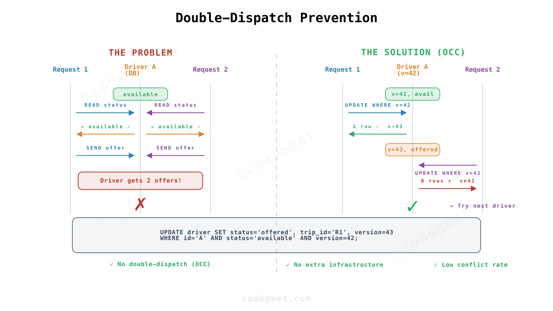
Approach 1: Optimistic Concurrency Control (Recommended)
Add a version field to each driver record. The reservation operation is a conditional write:
UPDATE driver
SET status = 'offered',
    current_trip_id = 'R1',
    version = 43
WHERE id = 'A'
  AND status = 'available'
  AND version = 42;

-- Request 1 executes first → 1 row affected. Driver A reserved.
-- Request 2 attempts → version is now 43, WHERE matches 0 rows.
-- Request 2 fails gracefully, tries next candidate driver.
This is optimistic because we assume conflicts are rare and handle them after the fact. In balanced markets, most drivers don't have two simultaneous offers — the conflict rate is low.
Note:
WHERE status = 'available'alone prevents the basic race. Theversionfield handles a subtler edge case: a driver goesavailable → offered → available → offeredin quick succession, and a stale retry from the first cycle lands during the second.
Approach 2: Distributed Lock (Redis with TTL)
Acquire a lock on the driver ID before checking availability. Use an in-memory store with a TTL matching the offer window (e.g., 15 seconds). Only one matching request can hold the lock at a time.
Caveats: lock acquisition adds a network round-trip. If the lock holder crashes, you wait for the TTL to expire. Without a fencing token, edge cases can still produce double-dispatch. Under high concurrency, many requests queue on the same lock.
Alternative: Single-Writer Pattern
Route all matching requests for a geographic zone to a single matching service instance. If only one process assigns drivers in Zone A, there are no concurrent conflicts by design.
This eliminates the race condition at the application level — no locks, no version checks. But it requires robust leader election plus fencing tokens to prevent split-brain scenarios. The single writer also becomes a bottleneck and a single point of failure.
This pattern works for small-scale systems or as an optimization within a geographic cell, but adds operational complexity.
Recommendation: Use optimistic concurrency as the default. It's the simplest, requires no additional infrastructure, and performs well when conflicts are rare — which they are for ride matching. Mention distributed locks as an alternative if asked about higher contention.
Handling the Offer Window
The conditional update reserves the driver by setting status to offered. During the 15-second offer window, no other request can claim them. If the driver accepts, status transitions to en_route_to_pickup. If they decline or time out, status returns to available (with a new version number) and the next candidate is tried.
<discuss-with-ai-button title="Double-Dispatch Prevention" context="Two riders simultaneously try to book the same nearby driver. Without protection, both see the driver as available and both send an offer. Optimistic concurrency control with a version field prevents this race condition." points='["Why is optimistic concurrency preferred over distributed locks for ride matching?","What happens if a driver goes available→offered→available→offered rapidly and a stale retry arrives?","How does the single-writer pattern trade simplicity for availability?","What is the expected conflict rate in a balanced market vs a hotspot?","How do you handle the edge case where a driver's app crashes mid-offer?"]'>
How do you estimate time of arrival for both pickup and destination?
ETA Estimation
The rider sees "Driver arriving in 4 minutes" and "Trip will take 23 minutes." These estimates affect the rider's decision to request and the driver's decision to accept. Inaccurate ETAs erode trust.
Approach 1: Straight-Line Distance
Calculate distance between two points, divide by average speed. Fast to compute. Limitation: ignores roads entirely. A 2km straight line might be 5km of winding streets.
Approach 2: Road Network Routing
Model the road network as a weighted graph: intersections are nodes, road segments are edges, weights are expected travel times. Shortest-path algorithm (Dijkstra or A*) finds the fastest route.
Raw edge weights come from speed limits, road type (highway vs residential), number of lanes. This gives a baseline ETA assuming free-flow traffic. Limitation: free-flow ETA is often wrong during rush hour. A 10-minute highway trip at 3am becomes 40 minutes at 5pm.
Approach 3: Traffic-Adjusted Routing (Recommended)
Adjust edge weights using real-time traffic data from multiple sources:
- Active drivers on the road — Drivers moving through the network report their speed via GPS updates. If 50 drivers on a highway segment average 20 km/h instead of the posted 100 km/h, that edge weight increases proportionally.
- Historical patterns — Traffic follows predictable patterns: rush hour, weekends, holidays. Historical data provides a baseline adjustment.
- External feeds — Traffic incidents, road closures, and construction from mapping data providers.
Pickup ETA vs Trip ETA
| Pickup ETA | Trip ETA | |
|---|---|---|
| What | Driver to rider | Pickup to destination |
| Accuracy | Must be accurate to within a minute | Can be less precise at request time |
| Why | Rider is actively waiting | Informational before trip starts |
| Improvement | Improves as driver approaches | Improves during trip with actual route data |
Learning from Completed Trips
After each trip, the system compares predicted ETA with actual travel time. This feedback loop improves future estimates. If the model consistently underestimates a road segment, the edge weight increases. ML models trained on millions of trips capture patterns that static routing misses: left turns at certain intersections take longer, school zones slow traffic at specific times.
Recommendation: Use traffic-adjusted routing. Road network graph with real-time edge weights from driver GPS data. Supplement with historical patterns for sparse-data scenarios. A bias toward slight overestimation creates a better UX than optimistic estimates that are frequently wrong.
How do you handle driver unavailability during matching?
Matching Resilience
The matching service found 5 nearby drivers sorted by distance. It sends an offer to Driver 1 (nearest). Driver 1 doesn't respond within 15 seconds. Now it tries Driver 2. Driver 2 declines. Driver 3 accepts — but in those 30 seconds, what has the rider experienced?
Approach 1: Sequential Cascading Offers
Try drivers one at a time, moving to the next on timeout or decline. Predictable and simple. Limitation: slow. If each candidate takes up to 15 seconds to time out, trying 5 drivers takes over a minute.
To speed this up, reduce the timeout window for subsequent candidates: First: 15s. Second: 10s. Third: 8s. Drivers who accept quickly are the ones you want.
Approach 2: Parallel Offers (Broadcast)
Send the offer to multiple drivers simultaneously. Accept the first response. The rider gets matched as soon as any driver accepts.
Limitation: if two drivers accept within milliseconds, one must be rejected. A two-phase offer/confirm flow or delayed navigation mitigates this.
Most production systems use a hybrid: send to 2-3 drivers simultaneously, accept the first, cancel the others.
Expanding Search Radius
If all candidates within the initial radius (~3km) decline, expand: 5km → 8km → maximum. The tradeoff: a driver 8km away means a long pickup time. Communicate the expected wait: "No nearby drivers. Expand search? Estimated pickup: 12 min."
Demand Queueing
During extreme demand (rainstorm, concert ending, New Year's Eve), every nearby driver may be occupied. Rather than "no drivers available," the system can queue the request and match as soon as a driver completes a nearby trip.
The rider sees: "High demand. Estimated wait: 5 min." When a nearby driver completes a trip, the system immediately offers them the queued request before they appear as "available" to new searches. This reduces wait time because drivers don't sit idle between trips.
This is where surge pricing intersects with matching: higher prices during demand spikes incentivize more drivers to go online and some riders to wait, naturally balancing supply and demand.
Recommendation: Use hybrid parallel offers (2-3 candidates) with decreasing timeout windows. Add demand queueing for peak periods. Communicate wait times transparently — riders prefer honest estimates over uncertain waiting.
Staff-Level Discussion Topics
The following topics contain open-ended architectural questions without prescriptive solutions. They are designed for staff+ conversations where you demonstrate systems thinking, trade-off analysis, and strategic decision-making.
Surge Pricing and Demand-Supply Balancing
Context: It's Friday evening and it starts raining downtown. Ride requests spike 5× while available drivers drop. Wait times climb from 3 to 15 minutes. How do you balance supply and demand dynamically?
Discussion Points:
- Surge pricing mechanics: define geographic zones, compute supply/demand ratio per zone, apply a multiplier when demand exceeds supply
- Zone granularity tradeoff: too fine-grained and prices fluctuate block-by-block; too coarse and surge doesn't reflect local conditions
- Feedback loop dynamics: higher prices discourage some riders (reducing demand) and incentivize more drivers to enter the zone (increasing supply). How quickly does this equilibrate?
- Fairness concerns: should there be a cap? Should frequent riders get surge protection?
- Driver gaming: drivers may cluster at surge boundaries or go offline briefly to trigger higher surge. How to detect and mitigate?
<discuss-with-ai-button title="Surge Pricing and Demand-Supply Balancing" context="It's Friday evening and it starts raining downtown. Ride requests spike 5× while available drivers drop. Wait times climb from 3 to 15 minutes. How do you balance supply and demand dynamically?" points='["Surge pricing mechanics: define geographic zones, compute supply/demand ratio per zone, apply a multiplier to fares when demand exceeds supply","Zone granularity tradeoff: too fine-grained and prices fluctuate block-by-block; too coarse and surge doesn't reflect local conditions","Feedback loop dynamics: higher prices discourage some riders and incentivize more drivers. How quickly does this equilibrate?","Fairness concerns: should there be a fare cap? Should frequent riders get surge protection?","Driver gaming: drivers may cluster at surge boundaries or go offline briefly to trigger higher surge. How to detect and mitigate?"]'>
Multi-City Deployment and Geo-Partitioning
Context: The service operates in 500 cities across 40 countries. Each city has different regulations, driver pools, and traffic patterns. A rider in Tokyo should never be matched with a driver in Osaka. How do you partition the system?
Discussion Points:
- Geographic partitioning: each city is an independent partition with its own geospatial index, matching service, and driver pool
- Data locality: keep driver locations and trip data in the region closest to the city. Only border cases or failover query adjacent partitions.
- Shared vs isolated infrastructure: user accounts are global (a rider can use the app in any city), but matching is local
- Regulatory compliance: different cities have different pricing caps, driver requirements, and data residency rules
- Scaling strategy: add a new city by spinning up a new partition. What's the minimum infrastructure per city?
Fraud Detection: Fake GPS, Ghost Rides, and Abuse
Context: A driver reports GPS coordinates that show them driving the route, but the rider is still standing at the pickup point. The trip completes, the rider is charged, but no ride actually happened. How do you detect and prevent this?
Discussion Points:
- GPS spoofing detection: compare driver's reported location against expected patterns (speed between updates, consistency with road network, cell tower triangulation)
- Ghost ride detection: cross-reference driver's and rider's location streams during the trip. If they diverge, flag for review.
- Collusion patterns: driver and rider collude for fake trips and incentive payouts. Detect via network analysis (same pair repeatedly, unusual patterns)
- Real-time vs batch detection: GPS spoofing can be caught in real-time; collusion networks require batch analysis over historical data
- False positive handling: legitimate scenarios look like fraud (rider exits early, driver detours for construction)
Beyond Nearest Driver: Optimizing the Matching Algorithm
Context: Nearest driver isn't always the best match. Driver A is 2km away but heading in the opposite direction. Driver B is 3km away but already driving toward the rider. Driver C is 2.5km away and their current trip ends near the pickup. How do you optimize?
Discussion Points:
- Multi-factor scoring: combine distance, heading direction, predicted acceptance probability, ETA, and driver rating into a match score
- Destination-aware matching: match drivers whose current trip destination is near the new pickup. Reduces deadhead miles and gets the rider picked up faster.
- Batch matching: collect requests over a short window (2 seconds) and solve a global assignment problem minimizing total wait time
- Learning from history: drivers who frequently decline certain trips can be deprioritized for those types
- Fairness constraints: pure optimization might always send premium requests to high-rated drivers, leaving new drivers with undesirable trips
Level Expectations
The following table summarizes what interviewers typically expect at each seniority level for ride-hailing system design.
| Dimension | |||
|---|---|---|---|
| Requirements | Identify core FRs: request a ride, track driver location, match rider to driver. Basic scale math (trips per day, location updates per second). | Define precise NFRs: sub-second matching latency, location update throughput requirements, consistency guarantees for driver assignment. | Challenge requirements — should matching optimize for nearest driver or predicted acceptance? How does pricing interact with matching? What consistency level is actually needed? |
| High-Level Design | Basic architecture: Rider App → API Gateway → Matching Service → Driver App, with a database for trips and locations. | Separate write path (location ingestion to in-memory index) from read path (proximity queries). Introduce WebSocket, trip state machine, and event-driven side effects. | Geo-partitioned deployment per city, hot/cold path separation, event sourcing for trip lifecycle, connection registry for WebSocket routing across instances. |
| Geospatial Design | Explain that 'find nearby' needs spatial indexing, not just lat/lng columns. Mention geohash or quadtree. | Compare geohash vs quadtree tradeoffs: fixed vs adaptive cells, update cost, query pattern. Explain 9-cell search and expanding radius. | H3 hexagonal grids for uniform-area cells, multi-resolution indexing based on driver density, cross-cell boundary handling. |
| Matching & Consistency | Find nearest driver, send offer, handle accept/decline. Basic understanding of no-double-assignment. | Prevent double-dispatch with optimistic concurrency (version-based conditional update). Handle timeouts with cascading offers. Tradeoff vs distributed locking. | Batch matching across concurrent requests, global optimization (minimize total wait time), marketplace dynamics and surge pricing integration. |
| Real-Time Communication | Mention rider needs to see driver location in real-time. Suggest polling or WebSocket. | Choose WebSocket with reasoning (bidirectional, low overhead). Design connection management: registry, reconnection, missed-event replay. | Connection Service scaling (millions of concurrent sockets), geographic routing, graceful degradation on instance failure, mobile-specific optimizations (battery, bandwidth). |
Interview Cheatsheet
Core Architecture in 60 Seconds
"Fare estimate → Routing Service computes distance and time. Rider enters destination, Routing Service models the road network as a weighted graph, returns distance and ETA. Fare = base + distance × rate + time × rate."
"Find drivers → geospatial index. Standard database queries can't handle proximity search at scale. Geohash converts 2D coordinates into 1D strings; query the cell and 8 neighbors. Drivers update their position every 4 seconds into an in-memory index."
"Match → offer/accept with optimistic lock. Rank nearby drivers by distance, send offer to nearest. Driver has 15s. On decline/timeout, try next. Optimistic concurrency (version-based conditional update) prevents double-dispatch."
"Real-time tracking → WebSocket + connection registry. Bidirectional persistent connections. Driver sends GPS → Location Service → forwards to rider via connection registry lookup. Rider sees driver move on map every 4 seconds."
"Trip lifecycle → state machine with outbox events. SEARCHING → MATCHED → ARRIVED → IN_PROGRESS → COMPLETED. Each transition is atomic with side effects (notifications, metering, payment) triggered via domain events."
Key Trade-offs to Mention
| Trade-off | Option A | Option B | When to Choose |
|---|---|---|---|
| Index storage | In-memory geospatial index | Persistent spatial DB | In-memory for 500K writes/sec; persistent for durability (hot/cold path split) |
| Spatial indexing | Geohash | QuadTree / H3 | Geohash for simplicity; H3 for uniform density adaptation |
| Concurrency | Optimistic locking | Distributed lock | Optimistic when conflicts are rare; locks when contention is high |
| Offer strategy | Sequential cascade | Parallel broadcast | Sequential for simplicity; parallel (2-3) for speed |
| Communication | WebSocket | SSE / Polling | WebSocket for bidirectional real-time; SSE/polling if infra doesn't support persistent connections |
| Event publishing | Direct publish | Outbox pattern | Outbox for guaranteed delivery; direct for lower latency when loss is acceptable |
Common Mistakes to Avoid
- ❌ Storing live driver locations in a relational database with durable writes — 500K writes/sec with WAL/fsync is impractical
- ❌ Using
SELECT * WHERE distance < Xwithout spatial indexing — full table scan on 2M rows per ride request - ❌ Ignoring the double-dispatch race condition — the interviewer will ask about it
- ❌ Using polling for real-time tracking — unacceptable latency and overhead at this scale
- ❌ Forgetting the outbox pattern — dual-write problem between DB and message queue is a classic distributed systems failure
- ❌ Designing a single global matching service — must be geo-partitioned per city/metro