typeahead
Introduction
A typeahead system — also called autocomplete or search-as-you-type — is one of the most ubiquitous features in modern software. Every time you type into Google, Amazon, Spotify, or VS Code's command palette, a typeahead system kicks in: it predicts the rest of the word or phrase you're typing, offers ranked suggestions in real time, and lets you select one without completing the full query.
The core challenge sounds simple — "given a prefix, return the top-K most relevant completions" — but at scale (billions of queries per day, hundreds of millions of unique search terms, sub-100ms latency requirements) it forces us to make nuanced decisions about:
- Data structure choice: Tries, prefix hash tables, or inverted edge-n-gram indexes — each with different write-cost, read-cost, and memory trade-offs.
- Ranking model: Popularity frequency, recency weighting, personalization, trending boosts.
- Update strategy: Batch (daily aggregation) vs. real-time (streaming frequency updates).
- Caching layers: Browser-level, CDN edge, and server-side caches — the read-to-write ratio in typeahead is extreme (~1000:1), making caching critical.
- Fault tolerance at the edge: The typeahead endpoint is called on every keystroke — if it goes down or slows down, every user in the product sees the impact immediately.
In this editorial we design a Typeahead / Autocomplete System for a large-scale e-commerce platform from first principles. We derive every decision from the requirements, work through the math, implement the core data structure, and stratify depth by seniority level so you can tailor your interview answers precisely.
Functional Requirements
We decompose functional requirements from the verbs in the problem statement:
Core (must-have for MVP)
- Suggest — As the user types each character, the system must return the top 10 most relevant search suggestions that match the current prefix, within 200ms.
- Rank — Suggestions must be ordered by a relevance signal (primarily popularity / search frequency, optionally weighted by recency).
- Update — The suggestion corpus must be updated at least daily to reflect new products, trending searches, and changing popularity.
- Store — The system must maintain a searchable index of all known search terms with their frequency scores.
Extended (out of scope but worth mentioning)
- Personalized suggestions (based on user's search/purchase history).
- Spell correction / fuzzy matching for typos.
- Trending/breaking suggestions (real-time boost for viral products).
- Multi-language / i18n support.
- Query categorization ("did you mean product, brand, or category?").
Non-Functional Requirements
Non-functional requirements come from the adjectives in the problem statement:
| Requirement | Target | Reasoning |
|---|---|---|
| Scale | 100M daily active users (DAU) | Large e-commerce platform |
| Read QPS | ~230K queries/sec (peak ~460K/sec) | Each keystroke triggers a request |
| Write volume | ~40 GB new term data/day | 10% of queries are new terms |
| Latency (p99) | < 200ms end-to-end | Must feel instant for good UX |
| Availability | 99.99% (52 min downtime/year) | Typeahead is on every page |
| Consistency | Eventual (daily updates acceptable) | Read-only for clients; corpus refreshed in batches |
| Accuracy | Top-10 suggestions match user intent | Ranking quality matters more than absolute freshness |
A critical insight: typeahead is extremely read-heavy — the read:write ratio is roughly 1000:1. This means caching is not optional; it's the primary design lever. Every layer of the system should be optimized for reads.
Resource Estimation
Assumptions:
- 100M daily active users (DAU)
- 20 search queries per user per day
- Average query length: 10 characters → 10 prefix requests per query (one per keystroke)
- Each suggestion response: ~500 bytes (10 suggestions × ~50 bytes each)
- 10% of queries are unique/new terms
- Each term record: ~20 bytes (term + frequency)
Traffic Estimation
| Metric | Calculation | Result |
|---|---|---|
| Queries per user per day | 20 searches × 10 keystrokes | 200 prefix requests/user/day |
| Total daily requests | 100M users × 200 | 20 billion requests/day |
| Average QPS | 20B ÷ 86,400 sec | ~230,000 queries/sec |
| Peak QPS (2×) | 230K × 2 | ~460,000 queries/sec |
Storage Estimation
| Metric | Calculation | Result |
|---|---|---|
| Daily new terms | 100M × 200 × 10% | 2 billion new term entries/day |
| Daily new storage | 2B × 20 bytes | ~40 GB/day |
| Annual storage | 40 GB × 365 | ~14.6 TB/year |
| Unique terms (estimated) | After deduplication | ~50M unique terms |
| Index size (prefix hash table) | 50M terms × avg 5 prefixes × 200 bytes/entry | ~50 GB |
Bandwidth Estimation
| Metric | Calculation | Result |
|---|---|---|
| Response bandwidth | 230K QPS × 500 bytes | ~115 MB/sec (920 Mbps) |
| Request bandwidth | 230K QPS × ~20 bytes (prefix) | ~4.6 MB/sec |
Performance Bottleneck
The bottleneck is read QPS (460K/sec at peak), not storage or bandwidth. This drives the entire architecture toward aggressive caching and in-memory serving. A single Redis node handles ~100K reads/sec, so we need at least 5 shards just for the cache layer.
API Design
The typeahead system exposes a single, ultra-high-traffic read endpoint and a batch-oriented write path.
Called on every keystroke. Must be stateless, cacheable, and blazing fast.
Request:
GET /api/suggestions?q=har&limit=10
Host: suggest.ecommerce.com
X-Request-ID: req-9f3a2c
Response:
{
  "prefix": "har",
  "suggestions": [
    { "term": "harry potter", "score": 9850 },
    { "term": "hard drive", "score": 7200 },
    { "term": "harness", "score": 4100 },
    { "term": "harper lee", "score": 3800 },
    { "term": "harmonics", "score": 2900 }
  ]
}
Design decisions:
limitparameter defaults to 10, capped at 25. Clients can request fewer suggestions on small screens.- Score is exposed to let the client do client-side re-ranking (e.g., boost recently searched terms).
- Response is JSON for simplicity; at very high scale, Protobuf or Flatbuffers can reduce serialization overhead by ~3×.
- No authentication required — suggestions are public data. This allows CDN edge caching.
Internal-only endpoint called by the batch pipeline after aggregating new frequency data.
{
  "data_source": "s3://suggestion-data/2025-03-17/aggregated.parquet",
  "strategy": "blue-green",
  "target_cluster": "suggest-prod-us-east"
}
This triggers a background job that:
- Reads aggregated frequency data from S3.
- Builds a new prefix hash table (or trie) in memory.
- Warms the cache on the standby cluster.
- Performs a blue-green swap — traffic shifts from the old cluster to the new one with zero downtime.
High-Level Design
How does the system serve suggestions in real time?
This is the core architectural question. A user types a character, and within 200ms the system must return the top-10 ranked suggestions for the current prefix. At 230K QPS (peak 460K), the read path must be heavily optimized.
Consider a naive approach: store all terms in a PostgreSQL table with a B-tree index on term. For prefix search, run SELECT term, frequency FROM terms WHERE term LIKE 'har%' ORDER BY frequency DESC LIMIT 10.
Problems:
- Latency: Even with an index,
LIKE 'har%'is a range scan. At 50M+ terms, this takes 10–50ms per query. With 460K QPS, the DB would need thousands of cores. - QPS ceiling: A single PostgreSQL node handles ~5K–10K simple queries/sec. We need 460K.
- No ranking optimization: The DB must scan all matching rows to find the top-10 by frequency.
The solution: pre-compute and cache the results so that lookups are O(1) key-value reads.
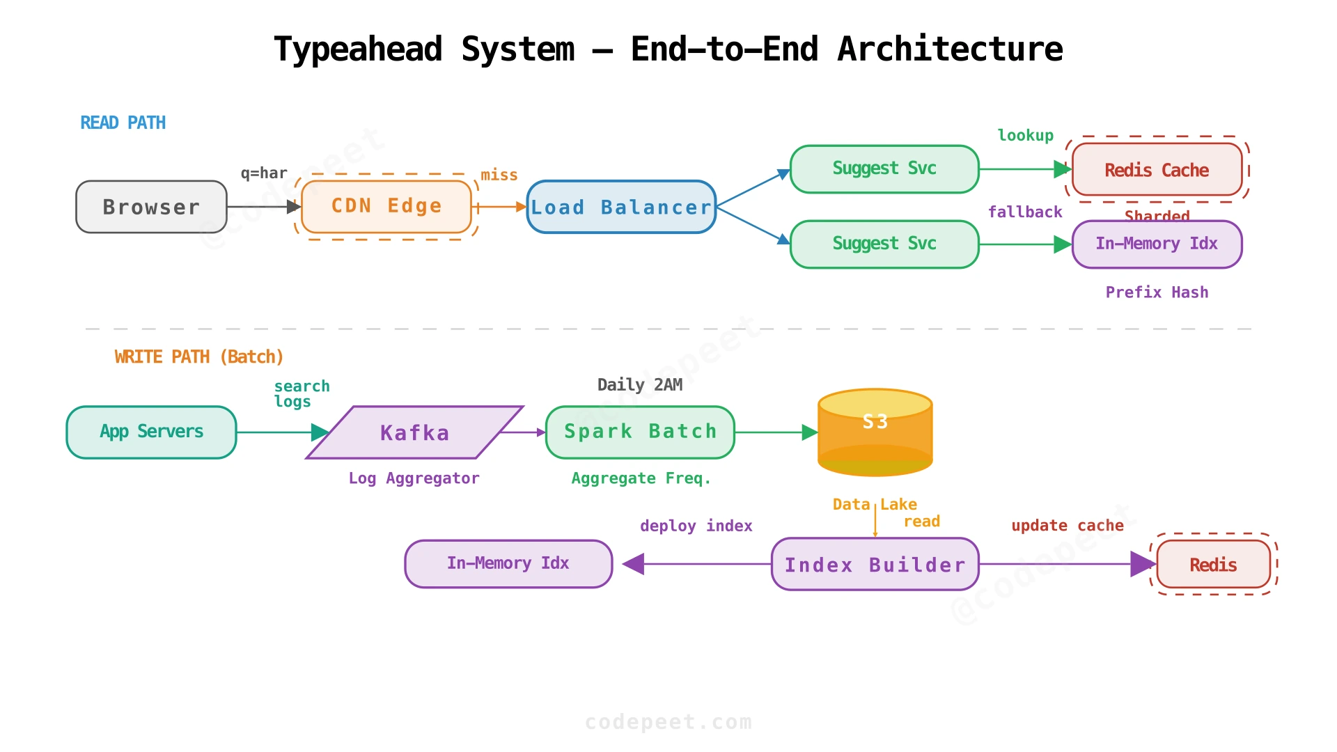
The architecture splits into two paths:
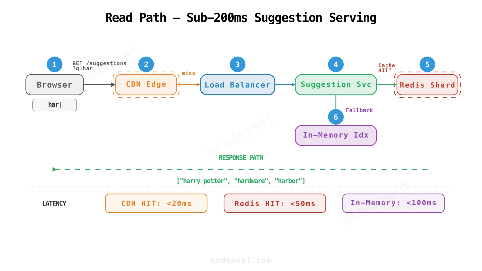
Read Path (latency-critical):
- User types a character → browser sends
GET /suggestions?q=<prefix>to the CDN. - CDN edge cache checks for an exact match on the prefix. Popular prefixes (top 1000: 'a', 'th', 'in', 'sh', ...) hit the CDN >90% of the time → response in <20ms.
- On CDN miss, the request reaches the Load Balancer which routes to a Suggestion Service instance.
- Suggestion Service checks the Redis cache cluster (sharded by prefix hash). Cache hit ratio is ~95% with a 24-hour TTL.
- On Redis miss, the service falls back to its in-memory prefix hash table — a local copy of the full index loaded at startup. This is the source of truth for suggestions.
- Response flows back through the LB and CDN (which caches it for subsequent requests).
Write Path (latency-tolerant):
- Application servers log every search query to a Kafka topic.
- A Spark batch job (runs daily or hourly) consumes the logs, aggregates term frequencies, and writes the output to S3 as a Parquet file.
- An Index Builder reads the aggregated data, constructs a new prefix hash table, and performs a blue-green deployment — warming the new index on standby nodes, then swapping traffic.
Typeahead is uniquely suited for CDN caching because:
- Prefix distribution follows Zipf's law: A small number of prefixes account for a huge percentage of traffic. The top 1,000 prefixes (
'a','the','sh','iph', ...) cover >50% of all requests. - Responses are identical for all users (no personalization in the base system). This means the same prefix always returns the same response, making it perfectly cacheable.
- Small response size (~500 bytes). CDNs can cache billions of small responses efficiently.
- TTL matches update frequency: If we rebuild the index daily, a 24-hour CDN TTL ensures users always see the latest suggestions while maximizing cache hit rate.
At-scale impact: With a 50% CDN hit rate, we cut origin QPS from 460K to 230K — effectively halving our infrastructure cost for the read path.
Before the request even leaves the browser, two optimizations dramatically reduce server load:
-
Debouncing: Don't fire a request on every keystroke — wait 100–150ms after the user stops typing. If a user types "harr" quickly, instead of firing 4 requests (
h,ha,har,harr), we fire 1 (harr). This can reduce QPS by 3–5×. -
Local result caching (browser memory): Store the last N prefix→suggestions mappings in a JavaScript Map. If the user types
har, gets results, then deletes therand retypes it, the secondharrequest is served from local memory — zero network latency.
Combined, debouncing + browser caching can reduce actual server QPS by 60–80% compared to the theoretical maximum.
How do we build and store the suggestion index?
The index is the heart of the typeahead system. Given a prefix, it must return the top-K results in O(1) or O(L) time (L = prefix length). We evaluate three approaches.
Approach 1: Trie (Prefix Tree)
A trie is a tree where each edge represents one character. A path from root to any node spells a prefix. Every node stores the frequency (or top-K results) for that prefix.
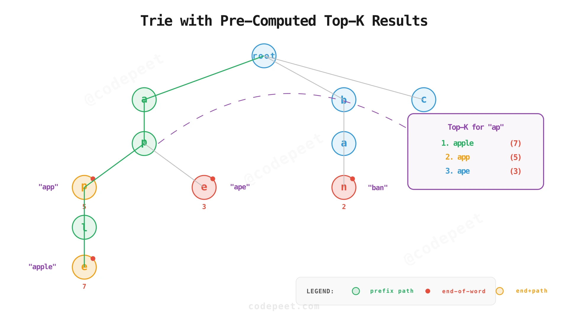
Naive trie: Store frequency only at leaf (end-of-word) nodes. To find top-K for prefix ap, traverse to the ap node, then DFS the entire subtree, collect all frequencies, sort, and return top-K. Time: O(L + N log N) where N is the subtree size.
Optimized trie: Pre-compute and store the top-K results at every node. Now lookup is O(L) — just traverse to the prefix node and return its pre-computed results.
class TrieNode:
    def __init__(self):
        self.children = {}       # char -> TrieNode
        self.top_words = []      # [(frequency, word), ...] sorted desc

    def update_top_k(self, word, frequency, k=10):
        # Update or insert the word in this node's top-K list
        for i, (freq, w) in enumerate(self.top_words):
            if w == word:
                self.top_words[i] = (frequency, word)
                self.top_words.sort(key=lambda x: (-x[0], x[1]))
                return
        self.top_words.append((frequency, word))
        self.top_words.sort(key=lambda x: (-x[0], x[1]))
        self.top_words = self.top_words[:k]


class Trie:
    def __init__(self):
        self.root = TrieNode()

    def insert(self, word, frequency):
        node = self.root
        for char in word:
            if char not in node.children:
                node.children[char] = TrieNode()
            node = node.children[char]
            node.update_top_k(word, frequency)

    def suggest(self, prefix):
        node = self.root
        for char in prefix:
            if char not in node.children:
                return []
            node = node.children[char]
        return [word for _, word in node.top_words]


# Example usage
trie = Trie()
trie.insert("apple", 5)
trie.insert("ape", 3)
trie.insert("app", 7)
trie.insert("apricot", 2)
print(trie.suggest("ap"))  # ["app", "apple", "ape", "apricot"]
Approach 2: Prefix Hash Table (Flattened Trie)
Instead of maintaining a tree in memory, we can flatten the trie into a key-value store where:
- Key: every possible prefix (e.g.,
'a','ap','app','appl','apple') - Value: the pre-computed top-K results for that prefix
{
  "a":   [{"term": "amazon", "score": 9500}, {"term": "apple", "score": 8200}, ...],
  "am":  [{"term": "amazon", "score": 9500}, {"term": "amd", "score": 3100}, ...],
  "ama": [{"term": "amazon", "score": 9500}, {"term": "amazon prime", "score": 7800}, ...],
  "ap":  [{"term": "apple", "score": 8200}, {"term": "app store", "score": 5600}, ...],
  "app": [{"term": "apple", "score": 8200}, {"term": "app store", "score": 5600}, ...]
}
With a prefix hash table, every suggestion lookup is a single O(1) hash table read — no tree traversal needed. This format maps perfectly to Redis or DynamoDB.
Trade-off: Trie vs. Prefix Hash Table
| Aspect | Trie (in-memory) | Prefix Hash Table (K/V store) |
|---|---|---|
| Lookup time | O(L) — traverse L characters | O(1) — single hash lookup |
| Memory | More compact (shared nodes) | Larger (duplicate top-K at every prefix) |
| Storage | RAM only (hard to persist) | Redis, DynamoDB, or any K/V store |
| Update | Rebuild trie in memory | Overwrite K/V entries in batch |
| Serialization | Complex (tree structure) | Trivial (JSON key-value pairs) |
| Use case | Single-node in-memory service | Distributed, cache-friendly architecture |
Recommendation: Prefix Hash Table for the production system. It's simpler to distribute, cache in Redis, replicate, and serve from CDN. The trie is useful for building the index in the batch pipeline, then it's flattened into a prefix hash table for serving.
Elasticsearch implements typeahead using edge n-gram tokenization. When indexing, each term is broken into all its prefixes:
"car"→ tokens:"c","ca","car""cat"→ tokens:"c","ca","cat"
The inverted index then maps each token to the documents (terms) containing it:
"c"   → ["car", "cat"]
"ca"  → ["car", "cat"]
"car" → ["car"]
"cat" → ["cat"]
This is conceptually identical to our prefix hash table — the difference is that Elasticsearch handles the infrastructure (sharding, replication, relevance scoring) out of the box. Good for rapid prototyping; less control over latency compared to a custom solution.
Deep Dives
The Data Pipeline — From Search Logs to Served Index
The write path is where raw user behavior becomes ranked suggestions. Unlike the read path (which must be sub-200ms), the write path is latency-tolerant — a daily batch run is perfectly acceptable for most typeahead systems.
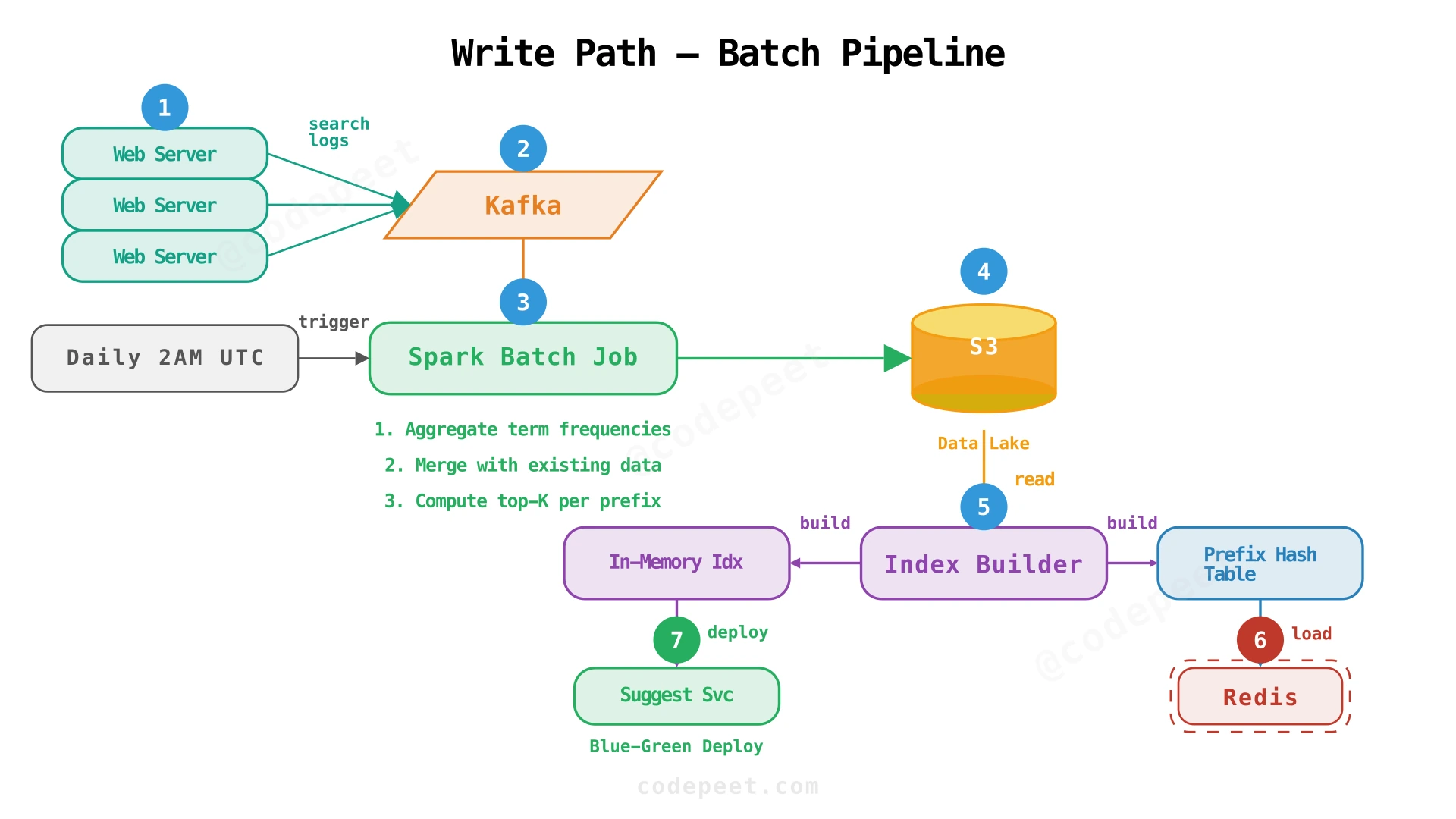
Pipeline stages:
-
Log Collection: Every search query is logged by the application servers. Logs are pushed to a Kafka topic (
search-queries) partitioned by date. -
Aggregation (Spark): A daily Spark job reads the last 30 days of search logs, deduplicates, and computes aggregate frequency for each unique term. Optionally applies time-decay weighting (more recent searches count more).
-
Frequency Table Construction: The Spark job outputs a Parquet file to S3 with schema:
(term: String, frequency: Long, last_searched: Timestamp) -
Prefix Hash Table Building: An Index Builder job reads the frequency table. For each term, it generates all prefixes and maintains a top-K list per prefix:
def build_prefix_hash_table(terms_with_freq, k=10):
    """Build a prefix -> top-K mapping from (term, frequency) pairs."""
    prefix_table = {}  # prefix -> [(freq, term), ...]

    for term, freq in terms_with_freq:
        for i in range(1, len(term) + 1):
            prefix = term[:i]
            if prefix not in prefix_table:
                prefix_table[prefix] = []
            bucket = prefix_table[prefix]
            bucket.append((freq, term))
            bucket.sort(key=lambda x: (-x[0], x[1]))
            prefix_table[prefix] = bucket[:k]

    return prefix_table


# Example
terms = [("apple", 8200), ("amazon", 9500), ("app store", 5600), ("amd", 3100)]
table = build_prefix_hash_table(terms)
print(table["ap"])
# [(8200, "apple"), (5600, "app store")]- Deployment (Blue-Green): The new prefix hash table is loaded into a standby Redis cluster and a standby set of suggestion service instances. Once warmed, traffic is switched from the active cluster to the standby — zero downtime.
The prefix hash table is large (~50 GB). Loading it into Redis or into in-memory indexes takes minutes. If we updated in-place, we'd have a window where:
- Some keys are from the old index, some from the new (inconsistent results).
- The loading process competes with serving traffic for CPU and memory.
Blue-green solves both: the standby cluster is fully loaded and warmed before any user traffic touches it. The swap is atomic — one DNS/LB config change.
Raw frequency (total searches all-time) has a problem: stale terms that were popular years ago dominate over currently trending terms. We apply exponential time decay:
Where is a decay constant and is days since last search. A typical gives a half-life of ~70 days — a term unsearched for 70 days has half its original weight.
In the Spark job, we compute this as:
import math
decay_lambda = 0.01
score = frequency * math.exp(-decay_lambda * days_since_last_search)
This naturally promotes trending terms while gracefully aging out stale ones.
Caching Strategy — Three-Layer Defense
With a 1000:1 read:write ratio and 460K peak QPS, caching isn't optional — it's the backbone of the read path. We implement a three-layer caching strategy.
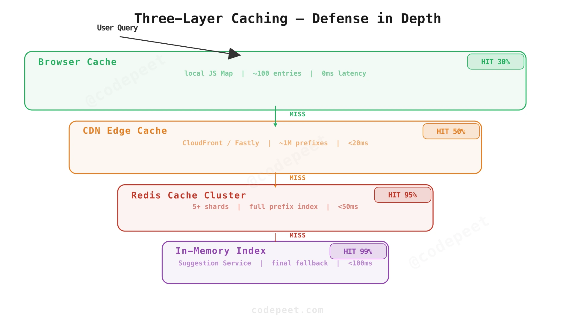
Layer 1: Browser Cache (Client-side)
The browser maintains an in-memory Map<prefix, suggestions[]> of the last 100 lookups. This primarily handles the backspace-retype pattern — user types har, deletes r, retypes r → cache hit on har.
Implementation: a simple JavaScript LRU cache with 100 entries.
Layer 2: CDN Edge Cache (CloudFront / Fastly)
Every GET /suggestions?q=... response has Cache-Control: public, max-age=86400. The CDN caches responses keyed by the full URL (including the q parameter). Popular prefixes (a, th, sh, in, iphone, ...) are served directly from the edge with sub-20ms latency.
- Expected hit rate: ~50% (Zipf distribution of prefix popularity).
- TTL: 24 hours (aligned with daily index rebuild).
Layer 3: Redis Cache Cluster (Server-side)
A sharded Redis cluster stores the full prefix hash table. Each shard is a Redis instance holding a subset of prefixes (sharded by consistent hashing on the prefix key).
- Expected hit rate: ~95% (only novel/rare prefixes miss).
- TTL: 24 hours (refreshed on each index rebuild).
- Memory: ~50 GB across 5 shards (10 GB/shard).
After a new index is built, the blue-green deployment warms the standby Redis cluster:
- Pre-load: The Index Builder writes all prefix→top-K pairs to the standby Redis cluster.
- Synthetic traffic replay: Replay the last hour of production requests against the standby to warm application-level caches and JIT compilation.
- Atomic swap: Once warm, the LB switches traffic to the standby cluster.
- CDN purge: Issue a CDN cache purge for
/suggestions*to ensure users see the updated suggestions.
No TTL-based invalidation is needed because we do a full cache replacement on every rebuild.
If the Redis cluster restarts or a new shard is added, all requests suddenly miss the cache and hit the in-memory index — a "thundering herd" on the suggestion services.
Mitigations:
- Request coalescing: If 100 concurrent requests for the same prefix all miss Redis, only one request is forwarded to the in-memory index; the other 99 wait for the result.
- Jittered cache TTLs: Add a random offset (±5%) to TTLs so entries don't all expire at the same time.
- Fallback circuit breaker: If Redis error rate exceeds 10%, bypass it entirely and serve from in-memory (which always has the full index).
Scaling to Billions of Queries
Our baseline: 100M DAU, 230K QPS, 460K peak. Let's examine how the system scales as the user base grows.
10× (1B DAU, 2.3M QPS peak 4.6M)
- CDN: Multiple CDN providers (CloudFront + Fastly) for geographic coverage. CDN hit rate becomes even more important — target 70%+ to keep origin QPS manageable.
- Redis: 50+ shards. Consider Redis Cluster with automatic failover.
- Suggestion Service: 100+ stateless instances behind the LB. Each instance loads the full in-memory index (~50 GB RAM). At this scale, the memory cost of having the full index on every instance becomes significant.
- Optimization: Tiered index loading: Each instance only loads prefixes for a subset (e.g., prefixes starting with a–m on one group, n–z on another). The LB routes by prefix range.
100× (10B queries/day — Google/Amazon scale)
- Custom infrastructure: At this scale, companies like Google build custom in-memory serving layers (Google's Suggest is served from custom C++ servers with memory-mapped trie structures).
- Multi-region: Deploy full read path stacks in every major region. The batch pipeline runs centrally, but the index is replicated to regional S3 buckets and loaded locally.
- Personalization: At this scale, personalized typeahead becomes valuable — combine global popularity with per-user history. This breaks CDN cacheability, so personalization happens at the service level, not CDN.
When the full index no longer fits on a single machine (or is wasteful to replicate), we shard by prefix range:
| Shard | Prefix Range | Approx. Size |
|---|---|---|
| Shard 0 | a* – d* | ~12 GB |
| Shard 1 | e* – j* | ~10 GB |
| Shard 2 | k* – p* | ~14 GB |
| Shard 3 | q* – t* | ~8 GB |
| Shard 4 | u* – z* | ~6 GB |
The load balancer routes GET /suggestions?q=har to Shard 2 (h is in k–p range). This reduces per-node memory by 5× while maintaining O(1) lookup.
Hot shards (a*, s*, c* are typically the busiest prefixes in English) get more replicas.
For a global product:
- Batch pipeline: Runs in a single region (us-east). Outputs the prefix hash table to S3.
- S3 replication: Cross-region replication to us-west, eu-west, ap-southeast buckets.
- Regional read stack: Each region has its own: CDN PoP → LB → Suggestion Service fleet → Redis cluster. Index is loaded from the local S3 bucket.
- DNS routing: Route53 latency-based routing sends users to the nearest region.
This gives sub-50ms latency globally while the write path remains centralized.
Typo Tolerance and Fuzzy Matching
Users make typos — aple instead of apple, amzon instead of amazon. A production typeahead system must handle these gracefully.
Approach 1: Edit-Distance Fuzzy Matching
For each prefix, compute the Levenshtein distance (insertions, deletions, substitutions) to all known terms and return those within a threshold (typically edit distance ≤ 2).
- Problem at scale: Computing edit distance against 50M terms for every keystroke is O(N × L) — far too slow.
- SymSpell optimization: Pre-compute all terms within edit distance 2 at index-build time. Store in a secondary hash table:
{"aple": ["apple"], "amzon": ["amazon"]}. Lookup is O(1) but the table is large.
Approach 2: Phonetic Matching (Soundex / Metaphone)
Map terms to phonetic codes. "smith" and "smyth" produce the same code. Useful for name searches but less effective for product/brand terms.
Approach 3: Character-level N-gram Overlap
Break the query and all terms into character bigrams. Rank by Jaccard similarity. Example: aple → {ap, pl, le}, apple → {ap, pp, pl, le}. Overlap = 3/4 = 0.75 → high match.
The most practical approach for our architecture: during the index build, generate fuzzy variants for each prefix:
- For each prefix of length ≤ 5 (where typos most commonly occur), generate all strings within edit distance 1.
- Map each variant to the same top-K results as the original prefix.
- Store these additional entries in the prefix hash table.
This increases the index size by ~5× for short prefixes but keeps lookup time at O(1). For longer prefixes (> 5 chars), typos are less common and the original prefix usually contains enough correct characters for a reasonable match.
def generate_edit_distance_1(prefix):
    """Generate all strings within edit distance 1 of the prefix."""
    alphabet = 'abcdefghijklmnopqrstuvwxyz0123456789 '
    results = set()
    # Deletions
    for i in range(len(prefix)):
        results.add(prefix[:i] + prefix[i+1:])
    # Substitutions
    for i in range(len(prefix)):
        for c in alphabet:
            results.add(prefix[:i] + c + prefix[i+1:])
    # Insertions
    for i in range(len(prefix) + 1):
        for c in alphabet:
            results.add(prefix[:i] + c + prefix[i:])
    results.discard(prefix)  # remove original
    return results
Typeahead fuzzy matching (during typing) is different from spell correction (after submission):
- Typeahead fuzzy matching: Must be fast (< 200ms), returns suggestions. Prefix-based.
- Spell correction: Can be slightly slower, corrects the full query. Uses Norvig's algorithm or a trained sequence-to-sequence model.
Google's approach: show typeahead suggestions while typing, and if the user submits a misspelled query, show "Did you mean: ..." on the results page — a separate system.
Staff-Level Discussion Topics
These open-ended topics have no single correct answer — they test architectural judgment and the ability to reason about complex trade-offs. Use the discussion buttons to practice articulating your thinking.
Global typeahead (same suggestions for everyone) is CDN-friendly and simple. Personalized typeahead ("you searched for 'python' before, so 'py' → 'python tutorial'" instead of 'PyTorch' for an ML engineer) is more useful but breaks cacheability.
Staff candidates should discuss:
- Hybrid approach: global top-7 + 3 personalized slots blended client-side.
- User embedding vectors: store a compact user preference vector, do real-time re-ranking at the service level.
- Privacy: personalized suggestions may leak sensitive search history.
Our design uses daily batch updates. But what if a major product launches or a celebrity endorsement goes viral? The term won't appear in suggestions until tomorrow's batch run.
Approaches to bridge the gap:
- Streaming layer: A Flink job reads the Kafka search log in real-time, maintains a sliding-window frequency counter, and pushes "trending" terms directly to Redis with a short TTL (1 hour).
- Lambda architecture: Batch pipeline for the stable base index + streaming pipeline for real-time delta. The suggestion service merges both at query time.
- Risk: Real-time updates can be gamed (bot search traffic to promote terms). Need rate limiting and anomaly detection on the streaming path.
Supporting typeahead in non-Latin scripts introduces unique challenges:
- Chinese/Japanese/Korean (CJK): No spaces between words. A user typing Chinese characters can't be prefix-matched the same way — need segmentation (word boundary detection) before indexing.
- Arabic/Hebrew: Right-to-left scripts. The prefix is built from the right side.
- Transliteration: Indian users may type Hindi words in Latin characters ("namaste" → suggest Hindi/Devanagari results).
- Index per language: Separate prefix hash tables per language to avoid cross-language pollution. The request includes an
Accept-Languageheader to route to the correct index.
Level Expectations
What interviewers expect at each seniority level for a typeahead system design:
| Area | |||
|---|---|---|---|
| Requirements | Lists FR (suggest, rank) and basic NFRs (fast, scalable) | Derives math: 230K QPS, 460K peak; identifies read-heavy ratio 1000:1 | Discusses personalization, real-time trending, multi-language as extensions |
| Data Structure | Knows trie exists for prefix search | Explains optimized trie with pre-computed top-K; compares trie vs. prefix hash table | Discusses edge n-grams, Elasticsearch integration, and when to build custom vs. use off-the-shelf |
| API Design | GET /suggestions?q=prefix | Explains CDN cacheability (public, max-age); debouncing at client | Designs internal rebuild API with blue-green strategy |
| Architecture | Client → Server → DB | Full read path: CDN → LB → Service → Redis → In-Memory; batch write path: Kafka → Spark → S3 → Index | Multi-region topology; tiered index loading; streaming + batch Lambda architecture |
| Caching | "Use Redis" | Three-layer strategy (browser, CDN, Redis) with hit rate analysis | Cache warming, avalanche prevention, request coalescing, jittered TTLs |
| Scaling | "Add more servers" | Redis sharding, suggestion service horizontal scaling | Prefix-range sharding, multi-region deployment, personalization at scale |
| Data Pipeline | "Build the trie from data" | Full batch pipeline: Kafka → Spark → S3 → Index Builder → Blue-Green deploy | Time-decay weighting, real-time trending layer, pipeline monitoring |
| Fuzzy Matching | Mentions Levenshtein distance | Explains SymSpell pre-computation; fuzzy prefix table approach | Discusses trade-offs: index size 5× vs. query-time fuzzy; phonetic vs. edit distance |
Interview Cheatsheet
Quick-reference talking points for the interview:
"A typeahead system returns ranked search suggestions as the user types each character. The core challenge is serving sub-200ms prefix lookups at 460K QPS peak. The architecture is a pre-computed prefix hash table served through a three-layer cache (browser → CDN → Redis), with a daily batch pipeline (Kafka → Spark → S3) rebuilding the index via blue-green deployment."
- FRs: Suggest (top-10 per prefix), Rank (by popularity), Update (daily batch), Store (prefix index)
- NFRs: 100M DAU → 230K QPS (peak 460K), < 200ms p99, 99.99% availability
- Read:Write ratio: 1000:1 → caching is the primary design lever
- Out of scope: Personalization, spell correction, real-time trending
- Browser — debouncing (100ms) + local LRU cache
- CDN Edge — caches prefix→suggestions (24h TTL, ~50% hit rate)
- Load Balancer — routes to suggestion service fleet
- Suggestion Service — stateless; reads Redis, fallback to in-memory index
- Redis Cluster — sharded prefix hash table (~50 GB, ~95% hit rate)
- Batch Pipeline — Kafka → Spark → S3 → Index Builder → Blue-Green deploy
- Index Builder — builds prefix hash table, warms standby cluster
- Trie vs. Prefix Hash Table: Trie is compact but hard to distribute; prefix hash table is O(1) lookup and maps to any K/V store
- Batch vs. Real-time updates: Batch is simpler and sufficient for daily freshness; streaming adds complexity but handles trending terms
- CDN cacheability vs. personalization: Global suggestions are perfectly cacheable; personalization breaks CDN caching
- Index size vs. fuzzy matching: Fuzzy prefix table increases index 5× but keeps lookup O(1)
- Blue-green deployment: Atomic index swap avoids partial-update inconsistency
| Metric | Value |
|---|---|
| DAU | 100M |
| Prefix requests/user/day | 200 (20 searches × 10 chars) |
| Average QPS | ~230K |
| Peak QPS (2×) | ~460K |
| p99 Latency target | < 200ms |
| Unique terms | ~50M |
| Index size (prefix hash table) | ~50 GB |
| CDN cache hit rate | ~50% |
| Redis cache hit rate | ~95% |
| Read:Write ratio | ~1000:1 |
- "How would you add personalization?" — Hybrid: global top-7 + 3 personal slots blended client-side. User preferences stored as embedding vectors in a fast K/V store.
- "What about real-time trending terms?" — Streaming layer (Flink) reads Kafka search logs, maintains a sliding-window counter, pushes trending terms to Redis with 1-hour TTL.
- "How do you handle offensive/sensitive suggestions?" — Blocklist filter applied at index build time. Emergency blocklist pushed to Redis as a separate key set; suggestion service filters results before returning.
- "How do you prevent abuse?" — Rate limiting per IP/user on the suggestion endpoint. On the write path, anomaly detection on search log frequencies to detect bot traffic.