google-map

Introduction

"Design Google Maps" is one of the most architecturally rich system design interview questions because it doesn't have a single dominant data flow — it's a multi-system composition problem. Unlike designing Twitter (one core feed pipeline) or Dropbox (one core sync pipeline), Google Maps requires you to orchestrate four fundamentally different subsystems, each with its own data model, scaling challenge, and algorithmic backbone:

Map Rendering — Serving pre-rendered image tiles at multiple zoom levels. This is a read-heavy CDN problem: billions of tile requests/day, served from edge caches.
Real-Time Traffic — Ingesting GPS pings from millions of devices, aggregating them per road segment, and producing live traffic overlays. This is a streaming analytics problem (Kafka + Flink).
Route Planning — Computing shortest/fastest paths across a massive road graph (billions of edges). This is a graph algorithm problem (Dijkstra, A*, contraction hierarchies).
Geo-Search — Finding nearby places (restaurants, gas stations, landmarks) given a location. This is a spatial indexing problem (geohash, quadtree, R-tree).

The interview challenge is that each subsystem could be a full design on its own. A strong candidate demonstrates breadth (knowing how the pieces fit together) and depth (diving into one or two subsystems with production-grade detail).

Google Maps serves 1 billion+ users, renders 100 million+ km of roads, and processes 50+ million route calculations daily. The map dataset is 20+ petabytes of imagery, terrain, and road data. This is one of the largest-scale consumer products ever built.

Functional Requirements

Core (must-have for MVP)

Map rendering — Display a navigable map with roads, buildings, water bodies, and terrain at multiple zoom levels (street → city → country → world). Pan and zoom must be smooth and responsive.
Real-time traffic — Show live traffic conditions as color-coded overlays on roads (green = free flow, yellow = moderate, red = heavy congestion).
Route planning — Given a source and destination, compute the shortest route (by distance) and the fastest route (by estimated travel time, accounting for real-time traffic).
Navigation — Provide turn-by-turn directions with real-time updates (rerouting if traffic changes or the user deviates from the planned route).

Extended (out of scope but worth mentioning)

Geo-search / POI (points of interest) — covered by Yelp system design.
Street View imagery.
Offline maps (download regions for use without connectivity).
Public transit / multi-modal routing.
Indoor mapping (airports, shopping malls).
Estimated time of arrival (ETA) prediction with ML.
Ride-sharing integration (Uber/Lyft overlay).

Non-Functional Requirements

NFR	Target	Reasoning
Scale	1 billion daily active users	Google Maps is one of the most-used apps globally
Read:Write ratio	1000:1	Overwhelmingly read-heavy (tile fetches, route queries); writes are GPS pings
Tile request QPS	~4 million/sec (average)	1B users × 360 tile loads/day ÷ 86,400
Route calculation QPS	~580/sec (average)	50M route calculations/day ÷ 86,400
GPS ingestion rate	~12 million pings/sec	1B active users sending location every ~5 seconds during navigation
Map tile latency	< 100ms (p99)	Users expect instant map rendering
Route calculation latency	< 500ms (p99)	Waiting more than a second for a route feels broken
Traffic overlay freshness	< 60 seconds	Traffic data older than a minute is misleading
Availability	99.99% (four nines)	Navigation is safety-critical (people rely on it while driving)
Storage	20+ PB	Satellite imagery, terrain data, road graphs, POI data
Global reach	Multi-region deployment	Users in Tokyo need low-latency tile serving, not from a US data center

Key insight: Google Maps has two fundamentally different data planes:

Static plane: Map tiles (imagery, roads, buildings) — changes infrequently (updated weekly/monthly), served from CDN. This is the easy part.
Dynamic plane: Traffic data, GPS pings, route calculations — changes every second, requires real-time streaming infrastructure. This is the hard part.

The architecture must cleanly separate these two planes because they have opposite scaling characteristics: static data is CDN-friendly; dynamic data is compute-intensive.

Resource Estimation

Assumptions:

1 billion daily active users
Average session: 30 minutes/user/day
Map tile request every 5 seconds during active use → ~360 tile requests/user/day
GPS location ping every 5 seconds during navigation (~20% of users navigating)
50 million route calculations/day
Average tile size: 30KB (compressed PNG at a given zoom level)
Data retention: 5 years for traffic history

Traffic Estimation

Metric	Calculation	Result
Daily tile requests	1B × 360	360 billion/day
Tile QPS (avg)	360B ÷ 86,400	~4.2 million/sec
Tile QPS (peak, 3×)	4.2M × 3	~12.5 million/sec
GPS pings	200M navigating × 1 ping/5s	~40 million pings/sec peak
Route calculations (avg QPS)	50M ÷ 86,400	~580/sec
Route calculations (peak, 10×)	580 × 10	~5,800/sec

Storage Estimation

Metric	Calculation	Result
Map tile storage	~200M unique tiles × 22 zoom levels × 30KB avg	~130 TB (pre-rendered tiles)
Satellite imagery (raw)	Full Earth at high resolution	~10 PB
Road graph	~1 billion edges × 200 bytes/edge	~200 GB
Traffic history (5 years)	~100M road segments × 1 snapshot/min × 100 bytes × 5 years	~26 PB
Total		~36 PB

Bandwidth Estimation

Metric	Calculation	Result
Tile serving bandwidth	12.5M tiles/sec × 30KB	~375 GB/sec peak
GPS ingestion bandwidth	40M pings/sec × 50 bytes	~2 GB/sec

The tile serving bandwidth (375 GB/sec) is enormous — this is why CDN is not optional, it's the primary serving layer. Without CDN, you'd need ~30,000 servers just for tile serving. With CDN, 95%+ of tile requests are served from edge caches and never hit origin.

API Design

Google Maps has two distinct communication patterns:

REST/HTTP for request-response (tiles, routes, search) — stateless, cacheable.
WebSocket for real-time GPS pings — persistent, bidirectional, high-frequency.

Map Tile API

Tiles are identified by a (zoom, x, y) coordinate tuple — this is the standard Slippy Map tile naming convention used by Google Maps, OpenStreetMap, and Mapbox.

GET /api/tiles/{zoom}/{x}/{y}.png
Authorization: Bearer {api_key}

Response: [compressed PNG image, ~30KB]
Cache-Control: public, max-age=86400
Content-Type: image/png

// Zoom levels: 0 (whole world, 1 tile) to 21 (street level)
// At zoom level z, the world is divided into 2^z × 2^z tiles
// Zoom 0: 1 tile | Zoom 10: ~1M tiles | Zoom 21: ~4 trillion tiles

Routing API

Computes shortest and fastest routes between two points.

GET /api/route?src_lat={lat}&src_lon={lon}&dst_lat={lat}&dst_lon={lon}&mode=driving
Authorization: Bearer {api_key}

Response:
{
  "shortest_route": {
    "distance_km": 12.4,
    "duration_min": 18,
    "polyline": "encoded_polyline_string",
    "steps": [
      { "instruction": "Head north on 5th Ave", "distance_m": 200, "duration_s": 30 },
      { "instruction": "Turn right onto Broadway", "distance_m": 1500, "duration_s": 180 }
    ]
  },
  "fastest_route": {
    "distance_km": 14.1,
    "duration_min": 14,
    "polyline": "encoded_polyline_string",
    "steps": [...]
  }
}

Real-Time Location API (WebSocket)

Persistent connection for GPS pings during active navigation.

// WebSocket: ws://location.maps.example.com/ws
// Client → Server (every 5 seconds during navigation):
{
  "type": "location_update",
  "lat": 37.7749,
  "lon": -122.4194,
  "speed_kmh": 45,
  "heading": 270,
  "timestamp": "2025-03-17T14:30:00Z"
}

// Server → Client (when rerouting needed):
{
  "type": "reroute",
  "reason": "traffic_change",
  "new_route": { "polyline": "...", "eta_min": 16 }
}

Why WebSocket for location pings instead of HTTP polling?

During active navigation, the client sends GPS pings every 5 seconds and needs to receive rerouting updates in real-time. With HTTP, each ping would require a new TCP connection (overhead: ~100ms for TLS handshake + HTTP headers). With 200M concurrent navigating users sending pings every 5 seconds, that's 40M HTTP requests/sec — each with connection overhead.

WebSocket eliminates this: one persistent TCP connection per navigating user. Pings are tiny JSON payloads (~50 bytes) sent over an already-open connection. The server can also push rerouting notifications instantly without waiting for the next client poll.

For non-navigating users (just browsing the map), HTTP is fine — tile requests are stateless and cacheable.

How does the Slippy Map tile system work?

The world map is projected onto a square (Mercator projection) and recursively subdivided:

Zoom 0: 1 tile covering the entire world (256×256 pixels).
Zoom 1: 4 tiles (2×2 grid).
Zoom z: $2^z \times 2^z$ tiles.
Zoom 21: ~4.4 trillion tiles (street-level detail).

Each tile is a 256×256 pixel PNG image. The tile at (zoom, x, y) covers a specific geographic bounding box. When the user pans or zooms, the client calculates which tiles are visible and fetches only those tiles.

Tile coordinates from lat/lon:

$x = \lfloor \frac{lon + 180}{360} \cdot 2^z \rfloor$

$y = \lfloor \frac{1 - \ln(\tan(lat) + \sec(lat)) / \pi}{2} \cdot 2^z \rfloor$

This formula maps any (lat, lon) to the exact tile (x, y) at zoom level z. The client uses this to request only the visible tiles.

High-Level Design

We build the architecture incrementally, starting from the simplest possible design and evolving it as each new requirement exposes a fundamental limitation. Google Maps is unique because it requires four distinct subsystems — each step adds one.

Step 1: Naive Design — Server-Side Map Rendering

Starting Point

Starting point: The simplest map service. The client sends its viewport coordinates, the server renders a map image on-the-fly from raw geodata (roads, buildings, rivers) and returns the image.

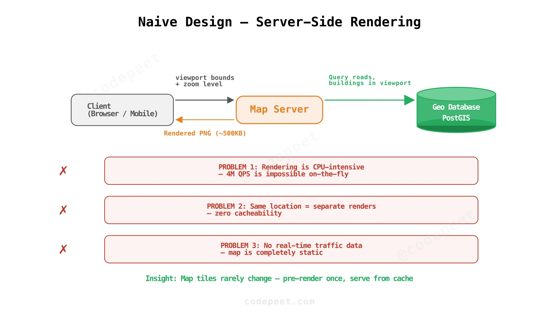
Naive design: client requests viewport, server renders map image on-the-fly

How it works:

Client sends its current viewport (bounding box + zoom level) to the Map Server.
Map Server queries the Geo Database for all features (roads, buildings, water, etc.) within the bounding box.
Map Server renders a PNG image from those features (using a rendering engine like Mapnik).
Returns the image to the client.

Three critical flaws:

Problem	NFR Violated	Impact
On-the-fly rendering	Latency, scale	Rendering a map tile takes 50-200ms of CPU. At 4M QPS, you'd need ~800,000 CPU cores.
No caching	Cost, latency	Two users looking at the same area get separately rendered images — identical work done twice.
No real-time traffic	Functionality	The map shows roads but not whether they're congested.

The fundamental insight: map tiles at a given zoom level rarely change (roads don't move). We should pre-render them once and serve from cache.

Step 2: Pre-Rendered Tiles + CDN — Solving Map Latency at Scale

Solving Scale and Latency

Problem being solved: On-the-fly rendering can't scale to 4M QPS. Users at the same location see the same map — we're wasting CPU re-rendering identical content.

Solution: Pre-render the entire world as a pyramid of tiles at 22 zoom levels. Store tiles as static PNG files. Serve through a CDN (Content Delivery Network) — edge caches around the world serve tiles with < 50ms latency, and 95%+ of requests never reach origin.

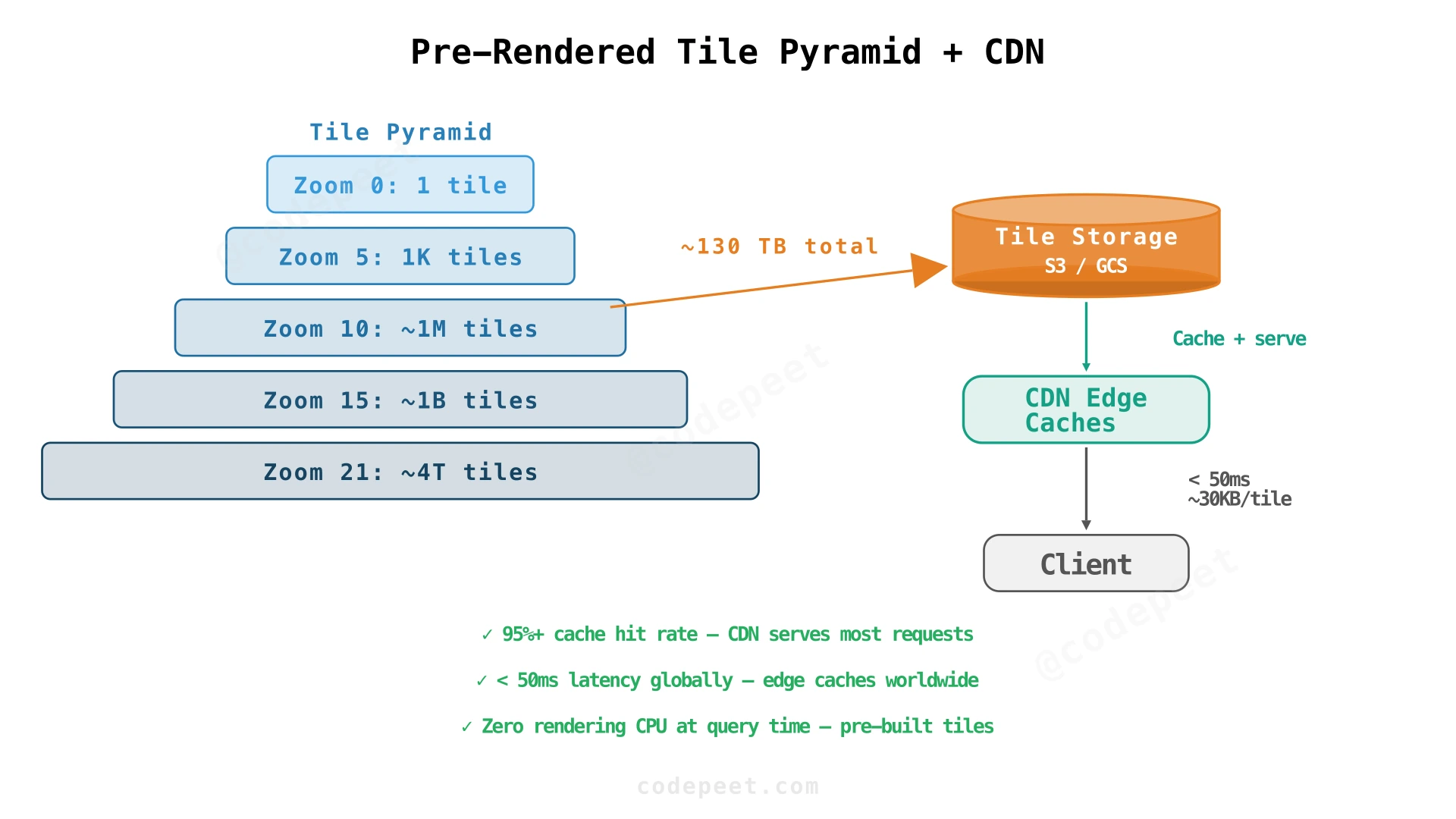
Tile pyramid: pre-rendered tiles at multiple zoom levels, served via CDN

How it works:

Offline pipeline: A batch rendering pipeline processes raw geodata (roads, buildings, water from OpenStreetMap or proprietary data) and produces PNG tiles for every (zoom, x, y) combination where there's meaningful content.
Tile storage: Tiles are stored in an object store (S3 / GCS). At 22 zoom levels, ~130 TB total.
CDN: Tiles are served through edge caches (Cloudflare, Akamai, Google's own CDN). Cache key = (zoom, x, y). TTL = 24 hours (tiles change infrequently).
Client: When the user pans or zooms, the client calculates which tiles are visible, fetches them from CDN, and assembles them into a seamless map.

Tile rendering is a batch job, not a real-time job. When road data is updated (new road built, name changed), the affected tiles are re-rendered and the CDN cache is invalidated. This happens weekly or monthly — not per-request.

What we've solved:

✅ Scale: CDN handles 12.5M peak QPS with no origin load.
✅ Latency: < 50ms from edge cache.
✅ Cost: Pre-render once, serve billions of times.

What's still broken:

❌ No real-time traffic: Tiles are static images — they don't know about current congestion.
❌ No routing: Users can see the map but can't get directions.
❌ No location tracking: No infrastructure for receiving GPS pings from users.

Why not vector tiles instead of raster (PNG) tiles?

Modern maps (including Google Maps since ~2013) use vector tiles instead of PNG tiles. Vector tiles contain raw geometry data (road paths, building polygons) in a compact binary format (Protocol Buffers). The client renders them using GPU-accelerated libraries (WebGL, Metal, Vulkan).

Feature	Raster (PNG) tiles	Vector tiles
Size	~30KB per tile	~10KB per tile (3× smaller)
Rendering	Server pre-renders	Client renders on GPU
Zoom	Discrete levels; blurry between levels	Smooth continuous zoom
Customization	Fixed style	Client-side styling (dark mode, custom colors)
Rotation	Labels rotate (look wrong)	Labels stay upright
Bandwidth	Higher	Lower

For the interview, either approach works. Mention vector tiles as a production optimization. The architectural pattern is the same: pre-generate tiles → store → CDN → client.

Step 3: Real-Time Traffic Pipeline — Live Congestion Data

Solving Traffic Freshness

Problem being solved: The map shows roads but not whether they're congested. Users need live traffic overlays updated within 60 seconds.

Solution: Build a streaming data pipeline that ingests GPS pings from millions of devices, aggregates them per road segment, computes traffic speed, and pushes color-coded traffic overlays to clients.

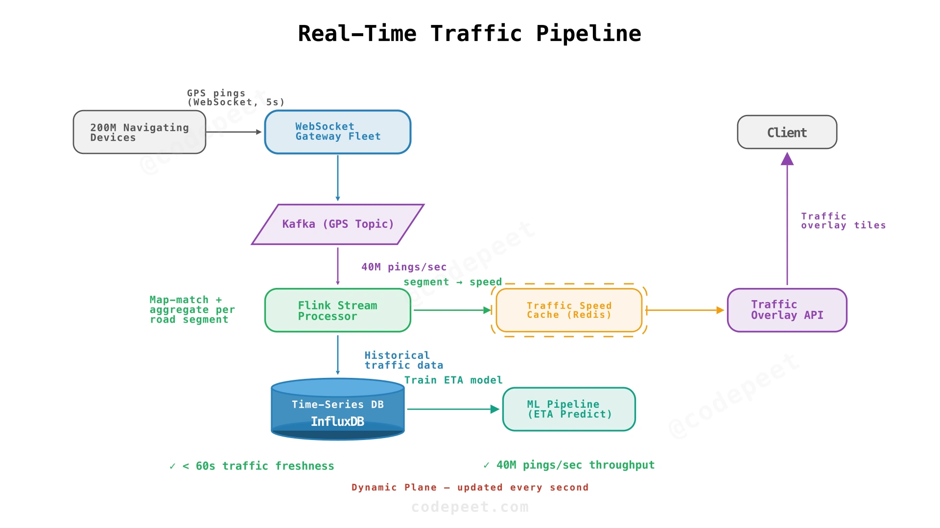
Real-time traffic pipeline: GPS pings → Kafka → Flink → traffic overlay

How the pipeline works:

GPS ingestion: 200M navigating users send GPS pings every 5 seconds via WebSocket. A fleet of stateless WebSocket gateways receives pings and publishes to Kafka.
Map matching: The Flink stream processor takes raw GPS coordinates and snaps them to the nearest road segment. Raw GPS is noisy (±10m accuracy) — map matching uses a Hidden Markov Model (HMM) to find the most likely road.
Speed aggregation: For each road segment, compute the average speed of all vehicles in the last 60 seconds. Classify: > 80% of speed limit = green, 40-80% = yellow, < 40% = red.
Cache update: Write {road_segment_id → speed, condition, timestamp} to Redis. This is the live traffic state.
Client overlay: Client polls the Traffic Overlay API (or receives push via WebSocket) with its visible road segments. API returns color codes from Redis.
Historical storage: All aggregated data also flows to a time-series database (InfluxDB) for historical analysis, ETA prediction, and ML training.

What we've solved:

✅ Live traffic: Color-coded overlays updated within 60 seconds.
✅ High throughput: Kafka + Flink handles 40M pings/sec.
✅ Historical data: Time-series DB supports ML-based ETA prediction.

What's still broken:

❌ No routing: Users can see traffic but can't get directions.
❌ Traffic data doesn't flow into route planning: The fastest route should use live traffic speeds.

How map matching works (snapping GPS to roads)

Raw GPS gives you coordinates like (37.7749, -122.4194) — but that's a point on the Earth, not a point on a road. The GPS might place you 10 meters into a building, or on the wrong side of a parallel road. Map matching solves this.

Simple approach (nearest road): Find the closest road segment to each GPS point. Fails when roads are close together (highway parallel to a service road).

Production approach (Hidden Markov Model):

States: Candidate road segments near each GPS point.
Emission probability: How likely is this GPS point given that the vehicle is actually on road R? (Based on distance from GPS point to road segment.)
Transition probability: How likely is moving from road R1 to road R2 between consecutive GPS points? (Based on road connectivity and distance traveled.)
Viterbi algorithm: Find the most likely sequence of road segments (the optimal path through the HMM).

This correctly handles ambiguous cases: if three GPS points in a row are near a highway, HMM will snap all three to the highway even if one point is slightly closer to a side street.

Step 4: Routing Service — Shortest and Fastest Path Computation

Solving Route Planning

Problem being solved: Users can see the map and traffic, but can't get directions. We need to compute shortest (by distance) and fastest (by time, using live traffic) routes.

Solution: Model the road network as a weighted graph where intersections are nodes and road segments are edges. Edge weights are distance (for shortest) or travel time (for fastest, using live traffic speeds from Redis). Use graph algorithms (Dijkstra/A*) with an optimization called segment-based caching that restricts computation to a relevant geographic area.

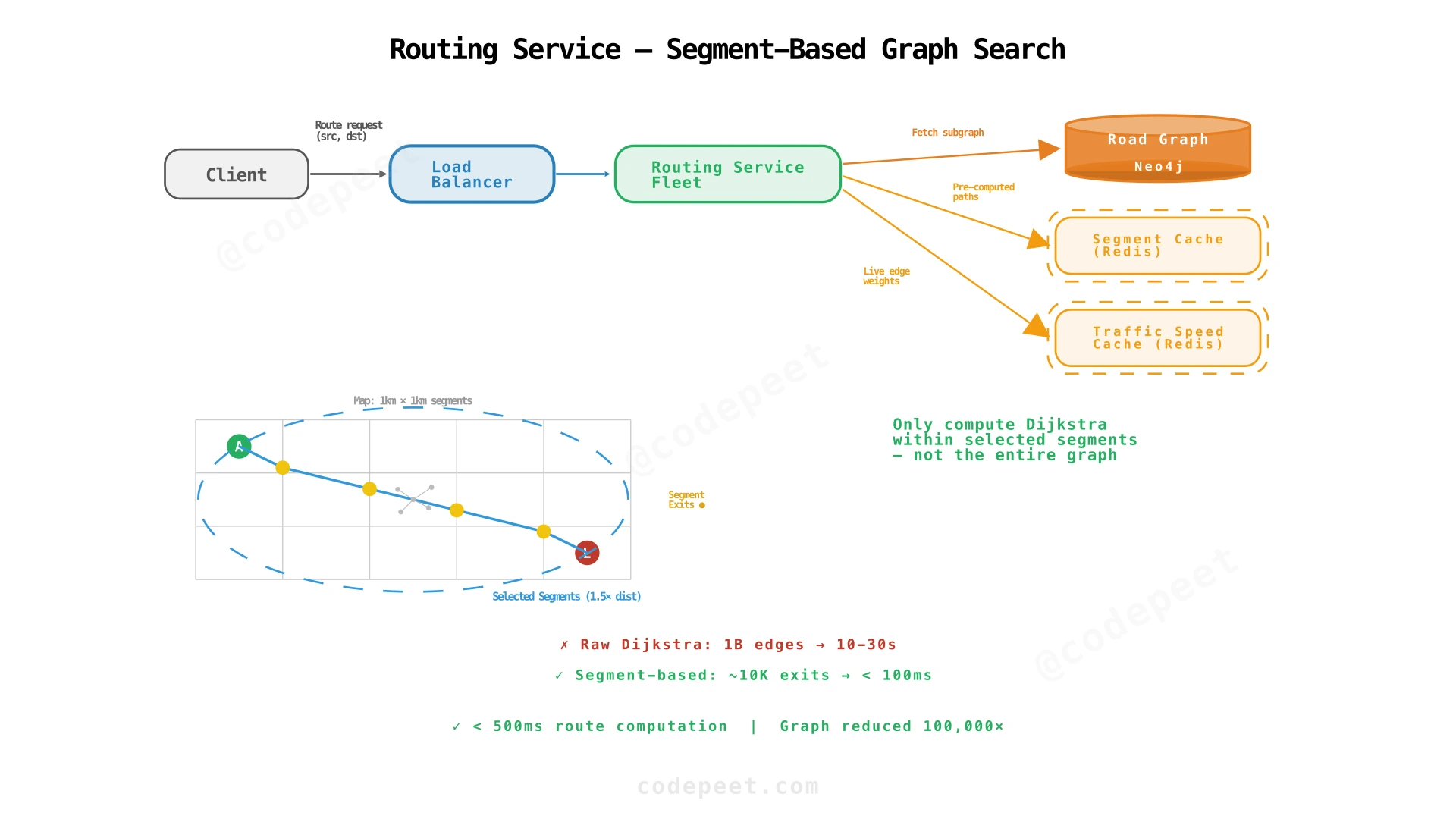
Routing service: road graph, segment caching, Dijkstra with live traffic weights

How routing works:

Step 1: Identify relevant segments
The map is divided into 1km × 1km segments. For a route from A to B, compute the straight-line distance and select all segments within 1.5× that distance. This limits the graph search to a small fraction of the total road network.

Step 2: Load subgraph
For each selected segment, load the pre-computed intra-segment shortest paths from Segment Cache (Redis). Each segment caches shortest paths between every pair of segment exits (points where roads cross segment boundaries).

Step 3: Construct inter-segment graph
Build a smaller graph where nodes are segment exits and edges are:

Intra-segment paths (from cache, weighted by distance or time).
Cross-segment connections (road crossing a segment boundary).

Step 4: Run Dijkstra/A*
Run Dijkstra's algorithm on this reduced graph. For shortest route, use distance weights. For fastest route, use live traffic speeds from the Traffic Speed Cache to compute travel time per edge.

Step 5: Return polyline
Convert the path of segment exits back to a detailed road polyline and return with turn-by-turn instructions.

Why segment caching is critical:

Approach	Graph size	Computation time
Raw Dijkstra on full graph	1 billion edges	10-30 seconds
A on full graph*	1 billion edges	2-5 seconds
Segment-based Dijkstra	~10,000 segment exits	< 100ms
Contraction hierarchies (Google's approach)	~100K shortcut edges	< 10ms

What we've solved:

✅ Route planning: Shortest and fastest routes computed in < 500ms.
✅ Live traffic integration: Fastest route uses real-time traffic speeds.
✅ Scalable: Segment caching reduces graph size by 100,000×.

What's still remaining:

❌ Segment cache invalidation: When traffic changes, intra-segment fastest paths must be recomputed.
❌ No unified architecture view: We haven't shown how all four subsystems connect.

Contraction Hierarchies — How Google actually does routing

While segment-based caching is a good interview answer, Google's production routing uses Contraction Hierarchies (CH) — a more sophisticated technique:

Offline preprocessing: Nodes are ordered by "importance" (small residential streets < highways). Less-important nodes are contracted by replacing them with shortcut edges between their neighbors.
Result: A hierarchical graph where long-distance paths use highway-level shortcuts and local paths use detailed street graphs.
Query: Bidirectional Dijkstra — one search from source (going up the hierarchy), one from destination (going up), meeting in the middle at highway-level nodes.
Speed: Queries take < 1ms on a graph with 50 million nodes (entire US road network).

The preprocessing is expensive hours on a large road graph) but done once. Queries are 100-1000× faster than plain Dijkstra.

Trade-off: CH assumes static edge weights. For live traffic (dynamic weights), Google uses a hybrid: CH for the highway backbone + local Dijkstra with live weights near source/destination.

Why a graph database (Neo4j) vs relational (PostgreSQL)?

The road network is inherently a graph: intersections are nodes, road segments are edges. Shortest-path queries are the core operation.

Database	Shortest path query	Storage efficiency	Ecosystem
Neo4j	Built-in Dijkstra/A* (GDS library)	Good for graph traversal	Graph-specific; limited for non-graph queries
PostgreSQL + pgRouting	Extension provides Dijkstra	Excellent for spatial data (PostGIS)	Full SQL ecosystem
Custom in-memory graph	Fastest; no DB overhead	Requires custom serialization	No ecosystem; full control

In practice, Google uses a custom in-memory graph engine (not Neo4j). For an interview, saying "graph database like Neo4j" or "in-memory graph" are both acceptable. The key insight is that the graph must fit in memory for fast pathfinding.

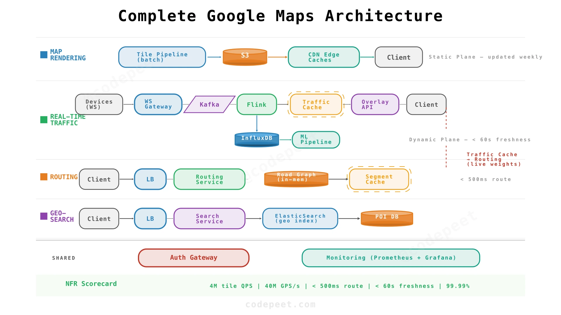
Step 5: Complete Architecture — All Subsystems Connected

Final Design

The complete architecture unifies all four subsystems under a coherent data flow with shared infrastructure (load balancers, monitoring, auth) and clear data dependencies between subsystems.

Complete Google Maps architecture with all four subsystems connected

NFR Scorecard — All Requirements Met

NFR	Target	How It's Achieved
1B DAU scale	Tile serving	CDN edge caches handle 12.5M peak tile QPS
< 100ms tile latency	CDN	95%+ cache hit rate; edge servers in every region
< 500ms route latency	Segment caching	Reduces graph from 1B edges to ~10K exits
< 60s traffic freshness	Kafka + Flink	Stream processing at 40M pings/sec with < 30s end-to-end
40M GPS pings/sec	WebSocket + Kafka	Stateless WS gateways; Kafka partitioned by geohash
99.99% availability	Multi-region	Each subsystem independently scaled + replicated
20+ PB storage	Tiered	CDN for tiles, S3 for imagery, InfluxDB for traffic history
Global reach	CDN + regional routing	Tiles from CDN; routing servers in every major region

Data Flow Dependencies

A key architectural insight: the four subsystems are not independent — they share data:

Traffic → Routing: Live traffic speeds (from Redis) feed into routing as dynamic edge weights.
Traffic → Tile overlay: Traffic conditions rendered as colored overlays on top of base tiles.
GPS → Traffic: Raw GPS pings are the input to the traffic pipeline.
Routing → Navigation: Route computation feeds turn-by-turn navigation.
GPS → Routing: Deviations from the planned route trigger re-routing.

These dependencies mean you can't just design four independent systems — you need shared infrastructure (Redis traffic cache, Kafka for GPS) and a coherent data flow.

Component summary and scaling strategy

Component	Responsibility	Scaling Strategy
Tile Rendering Pipeline	Batch-render map tiles from geodata	Horizontal MapReduce; weekly runs
Tile Storage (S3)	Store ~130 TB of tiles	Object store; region-replicated
CDN	Serve tiles at 12.5M peak QPS	Edge PoPs in 200+ cities globally
WebSocket Gateway	Receive GPS pings from navigating devices	Stateless; autoscale horizontally
Kafka	Buffer GPS pings + traffic events	Partitioned by geohash prefix
Flink	Map matching + speed aggregation	Parallel workers per Kafka partition
Traffic Speed Cache (Redis)	Live traffic state per road segment	Redis Cluster; sharded by road segment ID
Time-Series DB (InfluxDB)	Historical traffic data (5 years)	Time-based sharding + downsampling
Routing Service	Compute shortest/fastest paths	Stateless; in-memory graph loaded at startup
Road Graph (in-memory)	Weighted graph of all road segments	Sharded by geographic region
Segment Cache (Redis)	Pre-computed intra-segment paths	Invalidated when traffic data changes significantly
Search Service	Geo-search for POI	ElasticSearch with geospatial index

Why four separate databases?

Google Maps uses multiple specialized databases because each data type has fundamentally different access patterns:

Data Type	Database	Why
Spatial data (roads, buildings)	PostGIS (PostgreSQL)	Spatial indexes (R-tree), GIS functions
Road graph	Neo4j / Custom in-memory	Graph traversal (Dijkstra); adj-list access pattern
Traffic time-series	InfluxDB	Time-based queries, downsampling, retention policies
Live traffic state	Redis	Sub-ms reads; 40M writes/sec; TTL-based expiry
POI / search	ElasticSearch	Full-text + geospatial search, scoring

No single database excels at all of these. Using the right database for each workload is a core Google Maps design principle. This is called polyglot persistence.

Deep Dives

Database Design — Schema and Sharding Strategies

Deep Dive #1

Data Schema

Map Data (PostGIS):

-- Map tiles metadata
CREATE TABLE map_tiles (
  tile_id       TEXT PRIMARY KEY,        -- "z/x/y" e.g., "15/9650/12345"
  zoom_level    INT NOT NULL,
  bounds        GEOMETRY(POLYGON, 4326), -- geographic bounding box
  storage_url   TEXT NOT NULL,           -- S3/GCS URL for tile image
  last_rendered TIMESTAMPTZ,
  version       INT DEFAULT 1
);

-- Road segments (for traffic + routing)
CREATE TABLE road_segments (
  segment_id    UUID PRIMARY KEY,
  road_name     TEXT,
  road_type     TEXT NOT NULL,           -- highway, arterial, residential, etc.
  geometry      GEOMETRY(LINESTRING, 4326), -- road shape as ordered coordinates
  speed_limit   INT,                     -- km/h
  one_way       BOOLEAN DEFAULT FALSE,
  segment_key   TEXT                     -- 1km×1km segment identifier for partitioning
);
CREATE INDEX idx_road_geom ON road_segments USING GIST(geometry);

-- Landmarks / POI
CREATE TABLE landmarks (
  landmark_id   UUID PRIMARY KEY,
  name          TEXT NOT NULL,
  category      TEXT,                    -- restaurant, hospital, gas_station, etc.
  location      GEOMETRY(POINT, 4326),
  metadata      JSONB                    -- opening hours, ratings, photos, etc.
);
CREATE INDEX idx_landmark_geom ON landmarks USING GIST(location);

Traffic Data (Time-Series):

-- InfluxDB measurement (time-series)
-- measurement: traffic_speed
-- tags: road_segment_id, road_type, city
-- fields: avg_speed_kmh, vehicle_count, condition (green/yellow/red)
-- timestamp: auto

-- Example query: average speed on segment X in last 5 minutes
SELECT MEAN(avg_speed_kmh) FROM traffic_speed
WHERE road_segment_id = 'seg-abc123'
AND time > now() - 5m
GROUP BY time(1m)

Sharding Strategy

Data	Shard key	Why
Map tiles	`zoom_level` + geohash prefix	Tiles near each other geographically are served together; zoom levels have different access patterns
Road segments	`segment_key` (1km×1km grid ID)	Road segments in the same geographic area are queried together for routing
Traffic data	`road_segment_id` + time partition	Current data (hot) vs historical (cold); same road's data stays together
POI / Landmarks	Geohash prefix	Nearby POIs are queried together for geo-search
User data	`user_id` hash	Uniform distribution; user data accessed independently

Geographic sharding with geohash

Geohash encodes a (lat, lon) pair into a single string where shared prefixes indicate geographic proximity. For example:

9q8yyk = San Francisco, CA
9q8yy = broader SF area
9q8 = Northern California

Sharding by geohash prefix ensures that data for nearby geographic areas lands on the same shard — enabling efficient range queries ("all road segments in this area") without scatter-gather across all shards.

Hotspot mitigation: Popular areas (Manhattan, central Tokyo) have more data and traffic. Use a shorter geohash prefix for dense areas (more shards) and longer prefix for sparse areas (fewer shards). This adaptive sharding balances load.

ETA Prediction — From Heuristics to Machine Learning

Deep Dive #2

Estimated Time of Arrival is arguably the most user-facing metric in mapping — "how long until I get there?" The naive approach (distance ÷ speed limit) is wildly inaccurate. Production ETA requires multi-layered prediction.

Level 1: Speed limit based (naive)

Sum edge distances ÷ speed limit for each road segment.
Problem: Ignores traffic, traffic lights, turns, time of day.
Error: ±40-60%.

Level 2: Live traffic based

Use current average speed per road segment (from Traffic Speed Cache).
Problem: Assumes traffic stays constant during the entire trip. A 30-minute trip at 5 PM will encounter rush hour traffic that doesn't exist yet.
Error: ±15-25%.

Level 3: Historical + live (Google's approach)

Combine live traffic speed with historical traffic patterns for the same road, same day of week, same time.
For future segments of the route (20 minutes from now), use the historically predicted speed at that future time.
Error: ±5-10%.

Level 4: ML-based (Google DeepMind)

Google uses a Graph Neural Network (GNN) called ETA model that treats the road network as a graph and predicts travel time for each edge considering:
- Live traffic on the edge and neighboring edges
- Historical patterns (day/time/seasonal)
- Weather, events, road closures
- Time-dependent evolution (traffic 10 min from now)
Error: ±2-5% (published by Google in 2020 blog post).

How the ETA ML pipeline works in production

Feature engineering: For each road segment, compute features: current speed, speed 5/15/30 min ago, historical speed at this time/day, road type, # lanes, speed limit, weather, nearby event flags.
Graph Neural Network: The road network is the graph. Each node (intersection) has features from adjacent edges. The GNN propagates information across the graph — congestion on one road affects predicted speed on neighboring roads.
Route-level prediction: For a given route (sequence of edges), the model predicts total travel time. This is not just summing edge predictions — it accounts for interaction effects (e.g., a left turn at a busy intersection adds 60 seconds that per-edge models miss).
Serving: Model inference runs on TensorFlow Serving. Latency budget: < 50ms for ETA prediction (out of 500ms total route computation budget).

Real-Time Navigation and Rerouting

Deep Dive #3

Once a route is computed, the user begins navigating. The system must continuously monitor their position and reroute if conditions change.

Navigation loop (runs on the server every GPS ping):

Receive GPS ping — Device sends (lat, lon, speed, heading) every 5 seconds.
Map-match — Snap GPS to the nearest road on the planned route.
Progress check — Determine which step of the route the user is on. Update ETA.
Deviation detection — If the user has left the planned route (map-matched position is > 50m from route), trigger reroute.
Traffic change detection — Check if any road segment on the remaining route has significantly worsened (live speed dropped > 30% below predicted). If so, compute alternative route and compare ETA.
Push update — If rerouting, push new route via WebSocket. Otherwise, push updated ETA.

Rerouting decision logic:

IF deviation_from_route > 50 meters:
    → MANDATORY reroute (user missed a turn or took a different road)
ELIF new_route_saves > 2 minutes AND remaining_distance > 5 km:
    → SUGGEST reroute (don't annoy users with 30-second savings)
ELSE:
    → Continue current route, update ETA with live traffic

Challenges of rerouting at scale

With 200M concurrent navigating users, rerouting can cause a cascade problem: if traffic worsens on a highway, millions of users get rerouted to side streets, which then become congested, causing more rerouting... this is called oscillation.

Google's mitigation:

Stagger rerouting: Don't reroute all affected users simultaneously. Add random jitter (0-60 seconds) before triggering reroute checks.
Capacity-aware routing: Factor in the capacity of alternative routes. Don't send 10,000 cars down a residential street that can handle 200.
Predictive rerouting: Reroute before congestion hits (based on ML prediction), distributing cars across alternatives gradually instead of all at once.

Offline Maps — Downloading Regions for No-Connectivity Use

Deep Dive #4

Users in areas with poor connectivity (road trips, international travel) need offline maps. This requires downloading map tiles, road graph data, and POI for a selected region to the device.

Design:

Region selection: User selects a rectangular area on the map.
Package creation: Server computes which tiles (zoom 0-17), road graph edges, and POI fall within that region and creates a download package.
Incremental download: Package is split into chunks for resumable download. Delta updates for previously downloaded regions.
On-device routing: The device has a local routing engine that runs Dijkstra on the downloaded road graph. No server needed.
Sync on reconnect: When connectivity returns, the device syncs any missed updates (new POI, road changes).

Storage on device:

City (like San Francisco): ~150MB
Country (like Japan): ~1.5GB
Road graph for a city is small (~5MB); tiles are the bulk.

Compression techniques for offline maps

Vector tiles (not PNG) — 3× smaller and can be rendered on-device.
Reduced zoom levels — Offline often includes zoom 0-17 (not 18-21), cutting tile count significantly.
Graph compression — Road graph uses adjacency lists with varint encoding. Coordinate deltas (storing offset from previous point) compress well.
POI filtering — Only essential POIs (gas stations, hospitals, restaurants), not every bench and mailbox.

Staff-Level Discussion Topics

These open-ended topics test architectural judgment at the staff+ level.

Privacy vs. Traffic Quality Trade-off

Google Maps' traffic data comes from tracking user locations. More tracking = better traffic data. But users increasingly demand privacy. How do you maintain traffic quality while respecting privacy?

Multi-Modal Routing (Car + Transit + Walking)

Real-world navigation often combines modes: drive to the train station, take the train, walk to the destination. Multi-modal routing is fundamentally harder than single-mode.

Map Data Pipeline — From Satellite Imagery to Navigable Roads

Before any of this architecture works, someone has to create the map data. How does Google turn satellite imagery and street-level photography into a structured road graph with names, speed limits, turn restrictions, and lane markings?

Level Expectations

Area	Mid-Level	Senior	Staff
Requirements	Lists map rendering, routing, traffic	Derives 4M tile QPS, 40M GPS pings/sec; identifies static vs dynamic plane split	Discusses polyglot persistence, privacy vs traffic quality, capacity-aware routing
Architecture	Client → Server → Database	Four separate subsystems (tiles, traffic, routing, search); CDN for tiles; Kafka+Flink for traffic	Contraction hierarchies for routing; GNN for ETA; cascade prevention in rerouting
Map Tiles	"Serve map images"	Tile pyramid, zoom levels, CDN caching strategy, vector vs raster trade-off	Tile rendering pipeline (MapReduce), cache invalidation strategy, offline maps compression
Traffic	"Show traffic colors on roads"	Full streaming pipeline: GPS → Kafka → Flink → map matching → Redis; HMM for map matching	Differential privacy; k-anonymity; on-device aggregation; ML-based congestion prediction
Routing	"Use Dijkstra for shortest path"	Segment-based caching; reduced graph; live traffic weights; A* vs Dijkstra comparison	Contraction hierarchies; multi-modal routing; time-expanded graphs; Pareto-optimal routes
Database	"Use PostGIS"	Polyglot persistence (PostGIS + Neo4j + InfluxDB + Redis + ES); geohash sharding	Adaptive sharding for hotspots; time-series downsampling; cross-database consistency

Interview Cheatsheet

1. Opening Frame (30 seconds)

"Google Maps is a multi-system composition serving 1B+ DAU. Four core subsystems: (1) Map tiles — pre-rendered tile pyramid served through CDN at 12.5M peak QPS. (2) Real-time traffic — GPS pings from 200M navigating users flow through Kafka → Flink → Redis to produce live road speeds within 60 seconds. (3) Routing — road network modeled as a weighted graph; segment-based caching reduces 1B edges to ~10K exits for < 500ms computation. (4) Geo-search — ElasticSearch with geospatial index for POI queries. Key architectural insight: static plane (tiles, CDN-friendly) vs dynamic plane (traffic, compute-intensive) — these have opposite scaling characteristics and must be separated."

2. Requirements Scoping

FRs: Map rendering, real-time traffic, route planning (shortest + fastest), navigation with rerouting
NFRs: 1B DAU, 4M tile QPS, 40M GPS pings/sec, < 100ms tile latency, < 500ms route latency, < 60s traffic freshness, 99.99% availability
Key insight: Storage system (20+ PB) with a split personality — static (tiles) + dynamic (traffic). Separate them.
Out of scope: Street View, indoor mapping, public transit, ride-sharing integration

3. Core Architecture Components

Static plane (Map Tiles):

Tile Rendering Pipeline — batch MapReduce job; renders geodata → PNG/vector tiles
Tile Storage (S3) — ~130 TB of pre-rendered tiles
CDN — edge caches globally; 95%+ hit rate

Dynamic plane (Traffic + Routing):
4. WebSocket Gateway — receives GPS pings from navigating devices
5. Kafka — buffers GPS events; partitioned by geohash
6. Flink — map matching (HMM) + speed aggregation per road segment
7. Traffic Speed Cache (Redis) — live traffic state; sub-ms reads
8. Routing Service — in-memory graph; segment-based Dijkstra; live traffic weights
9. Time-Series DB (InfluxDB) — historical traffic; ML training data

Search plane:
10. Search Service + ElasticSearch — geospatial POI index

4. Key Trade-offs to Mention

Raster vs vector tiles: Raster simpler, vector smaller + client-rendered + smooth zoom
Long polling vs WebSocket for GPS: WebSocket wins — 200M persistent connections beat HTTP overhead
Graph DB vs in-memory graph: In-memory is faster; graph DB is more convenient. Google uses in-memory.
Dijkstra vs A vs contraction hierarchies*: Dijkstra is correct but slow; CH is 100-1000× faster but requires preprocessing
Live-only vs historical+live ETA: Historical patterns dramatically improve ETA accuracy for long trips
Geohash vs quadtree vs H3 for geo-sharding: Geohash is simplest; H3 has uniform cell sizes

5. Numbers to Remember

Metric	Value
DAU	1 billion
Tile request QPS (peak)	12.5 million
GPS ingestion rate (peak)	40 million pings/sec
Route calculations/day	50 million
Map tile storage	~130 TB
Total storage (imagery + roads + traffic history)	~36 PB
Tile latency (p99)	< 100ms (from CDN)
Route computation latency	< 500ms (segment caching)
Traffic freshness	< 60 seconds
CDN cache hit rate	95%+
Zoom levels	0-21 (22 total)
Tile size	~30KB (raster) / ~10KB (vector)
Road graph edges (global)	~1 billion

6. Possible Follow-up Questions

"How do you handle map updates (new roads)?" — Batch re-rendering of affected tiles; CDN cache invalidation; road graph edge addition with re-preprocessing of contraction hierarchies.
"How do you handle GPS noise?" — Hidden Markov Model map matching: candidates = nearby roads, emission = distance, transition = road connectivity, Viterbi decoding.
"How do you prevent rerouting oscillation?" — Stagger rerouting with random jitter; capacity-aware routing; predictive rerouting based on ML.
"How does offline maps work?" — Download tile + graph packages for region; on-device Dijkstra; delta sync on reconnect.
"How do you support multi-modal routing?" — Time-expanded graph; mode-switching edges; Pareto-optimal routes for competing objectives.
"How do you ensure privacy?" — Differential privacy on GPS; k-anonymity (k≥50) per segment; discard raw GPS after aggregation; on-device aggregation option.

Common Mistakes to Avoid

❌ Rendering map tiles on-the-fly per request — pre-rendered tiles served via CDN are the only way to achieve sub-100ms map loads
❌ Using a single flat grid for geospatial indexing — quad-trees or S2 cells handle variable density (urban vs rural) far better
❌ Running Dijkstra on the full road graph per route request — hierarchical preprocessing (contraction hierarchies) is necessary for sub-second routing at global scale
❌ Ignoring the read-to-write ratio — map tile reads outnumber traffic updates by 1000:1, so CDN caching is critical
❌ Not separating static map data from real-time traffic — static tiles change monthly, traffic data changes every minute; mixing them forces unnecessary tile regeneration
❌ Forgetting offline maps — navigation must work without connectivity, requiring downloadable tile + routing packages