realtime-monitoring-system
Introduction
Real-time monitoring systems are the nervous system of every modern infrastructure. Companies like Datadog, New Relic, Prometheus+Grafana, and AWS CloudWatch provide platforms that continuously ingest millions of metric data points per second from server fleets spanning thousands of machines, process those data points in real time to detect anomalies, trigger alerts, and render live dashboards that give engineering teams instant visibility into the health of their production environment.
In this editorial we design a Realtime Monitoring System from first principles — starting from requirements, estimating scale, choosing the right data pipeline, selecting a purpose-built time-series database, designing an alert-rule engine that evaluates streaming data, and finally building a dashboard service that can render both live and historical views.
The problem is deceptively simple on the surface — "collect metrics and show a dashboard" — but the real interview depth comes from:
- Metric ingestion at scale: How do you handle 6,000+ writes per second from 10K servers without overwhelming the database?
- Stream processing trade-offs: Push vs. pull, in-memory aggregation, statefulness.
- TSDB selection & schema: Why a time-series database beats RDBMS for this workload, and how to design an efficient schema.
- Alert rule evaluation: Real-time rule matching on streaming data — how to express threshold, rate-of-change, and composite conditions.
- Data tiering: Hot (seconds), warm (days), cold (months) — balancing granularity, cost, and query performance.
We derive every decision from the requirements, explain why each component exists, and stratify depth by seniority level so you can calibrate your interview answers precisely.
Functional Requirements
We decompose functional requirements from the verbs in the problem statement:
Core (must-have for MVP)
- Collect — The system must continuously collect server metrics (CPU, memory, disk, network I/O, and application-level counters) from a fleet of monitored servers at a configurable interval (default: every 10 seconds).
- Store — Collected metrics must be stored in a durable, queryable data store with configurable retention (e.g., raw data for 7 days, 1-minute aggregates for 30 days, 1-hour aggregates for 1 year).
- Alert — Users must be able to define alert rules (e.g., "avg CPU > 80% over 5 minutes") that are evaluated in real time. When a rule triggers, the system must deliver notifications via email, SMS, or push within 1 minute.
- Visualize — A web dashboard must display real-time and historical metrics with graphs, customizable time ranges, and per-server drill-down.
Extended (out of scope but worth mentioning)
- Log aggregation (system logs, access/error logs) — structurally similar pipeline.
- Distributed tracing integration.
- Anomaly detection with ML models.
- Auto-remediation (self-healing actions triggered by alerts).
Non-Functional Requirements
Non-functional requirements come from the adjectives in the problem statement:
| Requirement | Target | Reasoning |
|---|---|---|
| Scale | 10,000 servers initially; grow 20% annually | Typical mid-size fleet |
| Write throughput | ~6,000 metric writes/sec (peak ~18K) | 10K servers × 6 metrics ÷ 10s interval |
| Read throughput | ~60 reads/sec (dashboard queries) | 100:1 write:read ratio |
| Latency (ingest-to-dashboard) | < 30 seconds end-to-end | "Real-time" for monitoring purposes |
| Alert latency | < 1 minute from trigger condition to notification delivery | SLA for paging |
| Availability | 99.99% (52 min downtime/year) | Monitoring itself must be highly available |
| Durability | No metric loss during transient failures | Message queue buffers during DB downtime |
| Retention | Raw 7d → 1-min agg 30d → 1-hr agg 1yr | Balance granularity vs. storage cost |
| Cost | Minimize storage for cold data | Long-term storage on S3 or HDFS |
A critical insight: the monitoring system itself must be more reliable than the infrastructure it monitors — if your monitoring goes down during an outage, you're flying blind.
Resource Estimation
Assumptions:
- 10,000 monitored servers
- 6 metrics per server (CPU, memory, disk, network in, network out, app-level counter)
- Each metric point submitted every 10 seconds
- Each metric data point ≈ 100 bytes (server_id, timestamp, metric name, value, tags)
- Read-to-write ratio: 1:100 (dashboard queries are infrequent relative to ingest)
- Data retention: raw 7 days, 1-min aggregates 30 days, 1-hr aggregates 12 months
Traffic Estimation
| Metric | Calculation | Result |
|---|---|---|
| Writes/sec | 10,000 servers × 6 metrics ÷ 10 sec | 6,000 writes/sec |
| Peak writes/sec | 6,000 × 3 (peak factor) | ~18,000 writes/sec |
| Reads/sec | 6,000 ÷ 100 (read:write ratio) | 60 reads/sec |
| Daily data points | 6,000 × 86,400 sec/day | ~518 million/day |
Storage Estimation
| Metric | Calculation | Result |
|---|---|---|
| Daily raw storage | 518M points × 100 bytes | ~48 GB/day |
| Monthly raw storage | 48 GB × 30 | ~1.44 TB/month |
| Hot tier (raw, 7 days) | 48 GB × 7 | ~336 GB |
| Warm tier (1-min agg, 30 days) | 6× fewer points than raw | ~240 GB |
| Cold tier (1-hr agg, 12 months) | 360× fewer points | ~48 GB |
| Total hot + warm | 336 + 240 + 48 | ~624 GB |
| Cold (S3 long-term) | grows annually | ~1.4 TB/year |
Bandwidth Estimation
| Metric | Calculation | Result |
|---|---|---|
| Ingress bandwidth | 6,000 writes/sec × 100 bytes | ~600 KB/sec (4.7 Mbps) |
The write throughput is moderate — the challenge is not raw bandwidth but rather the number of individual writes (6K/sec steady, 18K/sec peak) and the need for real-time processing before storage.
API Design
We design three groups of APIs: metric ingestion, alert rule management, and metric querying.
The primary high-throughput API. Each monitored server's agent sends a batch of metric data points.
Request:
{
  "server_id": "srv-us-east-1-04821",
  "timestamp": "2025-03-17T14:30:00Z",
  "metrics": [
    { "name": "cpu_usage", "value": 72.5, "unit": "percent" },
    { "name": "memory_usage", "value": 61.3, "unit": "percent" },
    { "name": "disk_usage", "value": 45.8, "unit": "percent" },
    { "name": "network_in", "value": 12400, "unit": "bytes_per_sec" },
    { "name": "network_out", "value": 8700, "unit": "bytes_per_sec" },
    { "name": "active_connections", "value": 342, "unit": "count" }
  ],
  "tags": { "region": "us-east-1", "env": "production", "service": "api-gateway" }
}
Response: 202 Accepted (async ingestion — data is queued, not yet persisted)
{
  "status": "accepted",
  "batch_id": "b-7f3a9c2e"
}
Why 202 and not 200? The metric payload is written to a message queue (Kafka), not directly to the TSDB. The agent receives confirmation that the data was accepted for processing, not that it's already persisted. This decouples ingestion latency from storage latency.
Request:
{
  "name": "High CPU Alert",
  "metric": "cpu_usage",
  "condition": {
    "operator": "gt",
    "threshold": 80,
    "window": "5m",
    "aggregation": "avg"
  },
  "severity": "critical",
  "notify": ["email:oncall@company.com", "sms:+1234567890"],
  "filters": {
    "env": "production",
    "region": "us-east-1"
  }
}
Response: 201 Created with the rule ID.
Query parameters: metric, from, to, granularity (raw | 1m | 1h | 1d).
Response: Array of { timestamp, value } pairs for the requested metric and time range. The system automatically routes the query to the appropriate storage tier based on the time range and requested granularity — raw TSDB for recent data, aggregated tables for older data, and S3/HDFS for cold historical data.
High-Level Design
How do we ingest and process metrics at scale?
This is the core architectural question. We need to get 6,000 metric writes/sec (peak 18K) from 10,000 distributed servers into a time-series database, while simultaneously evaluating alert rules in real-time. The naive approach — agents writing directly to the TSDB — breaks down quickly due to peak traffic, transient failures, and the need for stream processing.
Consider InfluxDB as our TSDB. According to the official InfluxDB documentation, a cluster typically handles 5K–100K field writes per second depending on hardware. Our 6K requests/sec each carry 6 metric fields, giving us 36K field writes/sec at steady state and potentially 108K at peak. This pushes even a well-provisioned InfluxDB cluster to its limits.
More critically:
- No buffer during DB downtime: If the TSDB goes down for maintenance or fails, all incoming metrics are lost.
- No stream processing hook: We need to evaluate alert rules as data flows through, not after it's persisted.
- Tight coupling: Every agent needs to know the TSDB connection details, handle retries, and deal with backpressure.
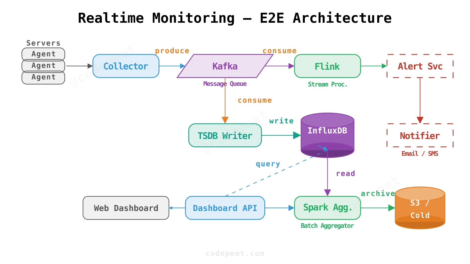
The architecture follows a "collect → queue → process → store → serve" pipeline:
-
Monitoring Agents — lightweight daemons installed on each server. They periodically sample hardware metrics (CPU, memory, disk, network) and tail log files for changes. Agents batch 10 seconds of metric data into a single payload and push it to the collector.
-
Collector / MQ Proxy — a stateless HTTP service that receives agent payloads, validates them, and publishes to Kafka. This decouples agents from Kafka's binary protocol and provides a stable API contract.
-
Message Queue (Kafka) — the central nervous system. Kafka topics are partitioned by
server_id(or region), providing:- Durability: Messages are replicated and persisted — if the TSDB is down, data waits in Kafka.
- Peak absorption: Kafka handles 2M+ writes/sec on three machines, easily absorbing our 18K/sec peaks.
- Fan-out: Multiple consumers (TSDB writer, stream processor, log indexer) can read independently.
-
Stream Processor (Flink/Storm) — a stateful consumer that reads from Kafka and:
- Evaluates alert rules against windowed metric data in real-time.
- Computes running aggregations (1-min, 5-min averages) in memory.
- Emits alert events to the notification pipeline when thresholds are breached.
-
TSDB Writer — a separate consumer that reads from Kafka and batch-writes metrics to the time-series database. Batching amortizes write overhead.
-
Time-Series Database (InfluxDB / TimescaleDB) — purpose-built for time-stamped data. Stores raw metrics for the hot tier (7 days).
-
Alert Service + Notification Service — receives alert events from the stream processor—deduplicates, applies cooldown/snooze logic, and dispatches via email, SMS, or push notifications.
-
Dashboard API — serves queries from the web UI. Routes to the appropriate storage tier based on the requested time range.
-
Batch Aggregator (Spark) — runs periodically to downsample raw data into 1-minute and 1-hour aggregates, then moves cold data to S3/HDFS for long-term retention.
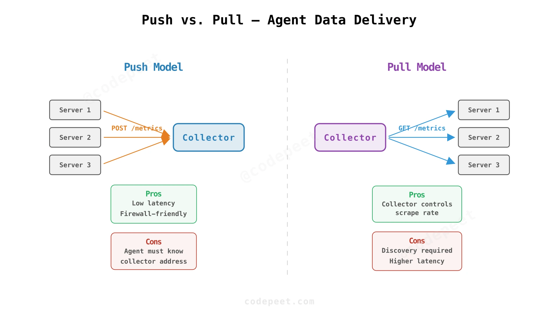
There are two fundamental approaches for getting metric data from agents to the collector:
| Aspect | Push (agent initiates) | Pull (collector polls agents) |
|---|---|---|
| Latency | Low — agent sends immediately | Higher — bounded by poll interval |
| Discovery | Agent must know collector address | Collector must discover all agents |
| Scale | Agents distribute load naturally | Collector must manage poll schedule for all targets |
| Firewall | Outbound from server (usually open) | Inbound to server (often blocked) |
| Failure handling | Agent retries locally | Collector must track which polls failed |
| Example | Datadog Agent, StatsD | Prometheus (pull-based scraping) |
Recommendation: Push model. For a monitoring system that requires near-real-time data with 10K+ servers, push is preferred because:
- Agents can batch and send asynchronously without waiting for polls.
- No central poll scheduler bottleneck.
- Works across firewalls and NATs without exposing server ports.
- Kafka naturally handles the firehose of push traffic.
However, Prometheus-style pull has advantages in environments where agent discovery is easy (Kubernetes service discovery) and where you want the collector to control the scrape rate. Many production systems use a hybrid: pull for Kubernetes pods, push for bare-metal servers.
Kafka topic design directly impacts parallelism and ordering guarantees:
Option 1: Partition by server_id — All metrics from a single server land in the same partition. This guarantees ordering per server (important if alert rules reference sequential data points). The stream processor can aggregate per-server metrics without cross-partition joins.
Option 2: Partition by metric name — All CPU metrics in one partition, all memory in another. This enables metric-specific processing pipelines but loses per-server ordering.
Option 3: Partition by region/environment tag — Coarse-grained. Useful for geographically distributed deployments where each region has its own processing pipeline.
Recommendation: Partition by server_id. With 10K servers and 32–64 Kafka partitions, each partition handles ~100–200 servers. This balances parallelism with per-server ordering. The partition key is a hash of server_id, so adding servers naturally distributes across partitions.
How do we store and query time-series data efficiently?
Time-series data has unique access patterns: writes are append-only and sequential in time, reads are almost always time-range scans, and recent data is accessed far more frequently than old data. A general-purpose RDBMS handles all of these poorly. We need a purpose-built time-series database.
Why TSDB over RDBMS?
| Feature | RDBMS (PostgreSQL) | TSDB (InfluxDB / TimescaleDB) |
|---|---|---|
| Write optimization | B-tree index updates on every insert | LSM tree / append-only — optimized for sequential writes |
| Compression | Row-based, moderate | Columnar + delta + gorilla encoding → 10–20× compression |
| Time-range queries | Full index scan or partition pruning | Native time-based partitioning, blazing fast range scans |
| Retention policies | Manual DELETE statements | Built-in retention policies with automatic drop |
| Downsampling | Manual aggregation queries | Continuous queries / materialized views built-in |
| Write throughput | ~5K–20K rows/sec (single node) | 50K–500K points/sec (single node) |
Database choice considerations:
InfluxDB:
- Purpose-built TSDB with its own query language (InfluxQL / Flux).
- Excellent write performance (100K+ field writes/sec per node).
- Built-in retention policies and continuous queries.
- Limitations: Custom query language (learning curve), HA requires enterprise edition.
TimescaleDB:
- PostgreSQL extension — full SQL compatibility.
- Automatic time-based partitioning (hypertables).
- Leverages PostgreSQL ecosystem (pg_dump, replication, extensions).
- Better for teams already running PostgreSQL who want SQL familiarity.
Prometheus TSDB:
- Designed for Prometheus's pull-based model.
- Excellent for Kubernetes-native monitoring.
- Limited long-term storage — typically paired with Thanos or Cortex for durable storage.
Recommendation for this design: InfluxDB (or TimescaleDB if SQL is preferred). InfluxDB gives us the highest raw write throughput and has built-in downsampling, while TimescaleDB is a strong choice if the team values SQL and PostgreSQL tooling.
Data Schema (TSDB — InfluxDB notation):
In InfluxDB's data model, data is organized into measurements, tags, and fields:
-- InfluxDB Line Protocol representation
-- measurement,tag_key=tag_value field_key=field_value timestamp

server_metrics,server_id=srv-04821,region=us-east-1,env=production
  cpu_usage=72.5,memory_usage=61.3,disk_usage=45.8,
  network_in=12400i,network_out=8700i,active_connections=342i
  1710686400000000000

-- Tags (indexed, low cardinality): server_id, region, env, service
-- Fields (not indexed, high cardinality values): cpu_usage, memory_usage, etc.
-- Timestamp: nanosecond precision Unix epoch
Relational Schema (PostgreSQL — for metadata, rules, alerts):
CREATE TABLE servers (
    server_id   VARCHAR(64) PRIMARY KEY,
    server_name VARCHAR(255) NOT NULL,
    region      VARCHAR(32) NOT NULL,
    environment VARCHAR(16) NOT NULL,   -- production, staging, dev
    created_at  TIMESTAMPTZ DEFAULT NOW()
);

CREATE TABLE alert_rules (
    rule_id     UUID PRIMARY KEY DEFAULT gen_random_uuid(),
    name        VARCHAR(255) NOT NULL,
    metric      VARCHAR(64) NOT NULL,   -- e.g., 'cpu_usage'
    operator    VARCHAR(4) NOT NULL,     -- gt, lt, gte, lte, eq
    threshold   DECIMAL(10,2) NOT NULL,
    window      INTERVAL NOT NULL,       -- e.g., '5 minutes'
    aggregation VARCHAR(8) NOT NULL,     -- avg, max, min, sum, p99
    severity    VARCHAR(16) NOT NULL,    -- info, warning, critical
    filters     JSONB DEFAULT '{}',      -- {"env": "production"}
    notify      TEXT[] NOT NULL,          -- ['email:x@y.com', 'sms:+1...']
    is_active   BOOLEAN DEFAULT TRUE,
    created_at  TIMESTAMPTZ DEFAULT NOW()
);

CREATE TABLE alerts (
    alert_id    UUID PRIMARY KEY DEFAULT gen_random_uuid(),
    rule_id     UUID REFERENCES alert_rules(rule_id),
    server_id   VARCHAR(64) NOT NULL,
    triggered_at TIMESTAMPTZ NOT NULL,
    resolved_at TIMESTAMPTZ,
    status      VARCHAR(16) NOT NULL DEFAULT 'open',  -- open, acknowledged, resolved
    metric_value DECIMAL(10,2) NOT NULL,  -- the value that triggered the alert
    created_at  TIMESTAMPTZ DEFAULT NOW()
);

CREATE INDEX idx_alerts_status ON alerts(status) WHERE status != 'resolved';
CREATE INDEX idx_alerts_rule ON alerts(rule_id, triggered_at DESC);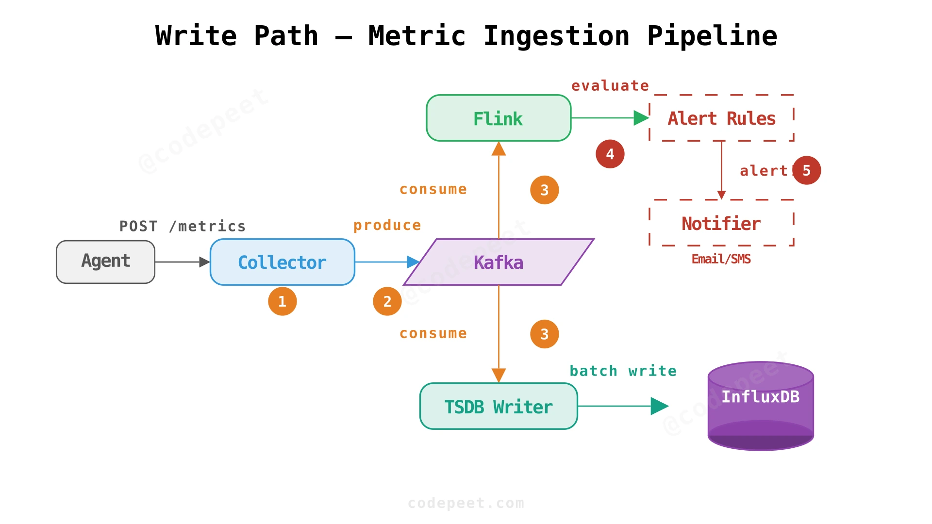
Partitioning:
Time-series data is naturally partitioned by time. Both InfluxDB and TimescaleDB support automatic time-based partitioning:
- Time-based shards (InfluxDB): Data is divided into "shard groups" by time interval (e.g., 1 day). Old shards can be dropped as a unit when the retention policy expires — this is O(1) file deletion, not row-by-row DELETE.
- Hypertable chunks (TimescaleDB): Similar concept, with automatic chunk creation.
For cross-server distribution, we can additionally partition by server_id hash or region tag to spread write load across multiple TSDB nodes.
Replication:
- Within a data center: synchronous replication (2 replicas) for strong consistency.
- Across data centers: asynchronous replication for disaster recovery.
- InfluxDB Enterprise provides built-in clustering. For OSS InfluxDB 2.x, we'd need to manage replication at the Kafka level (multiple consumer groups writing to separate DBs).
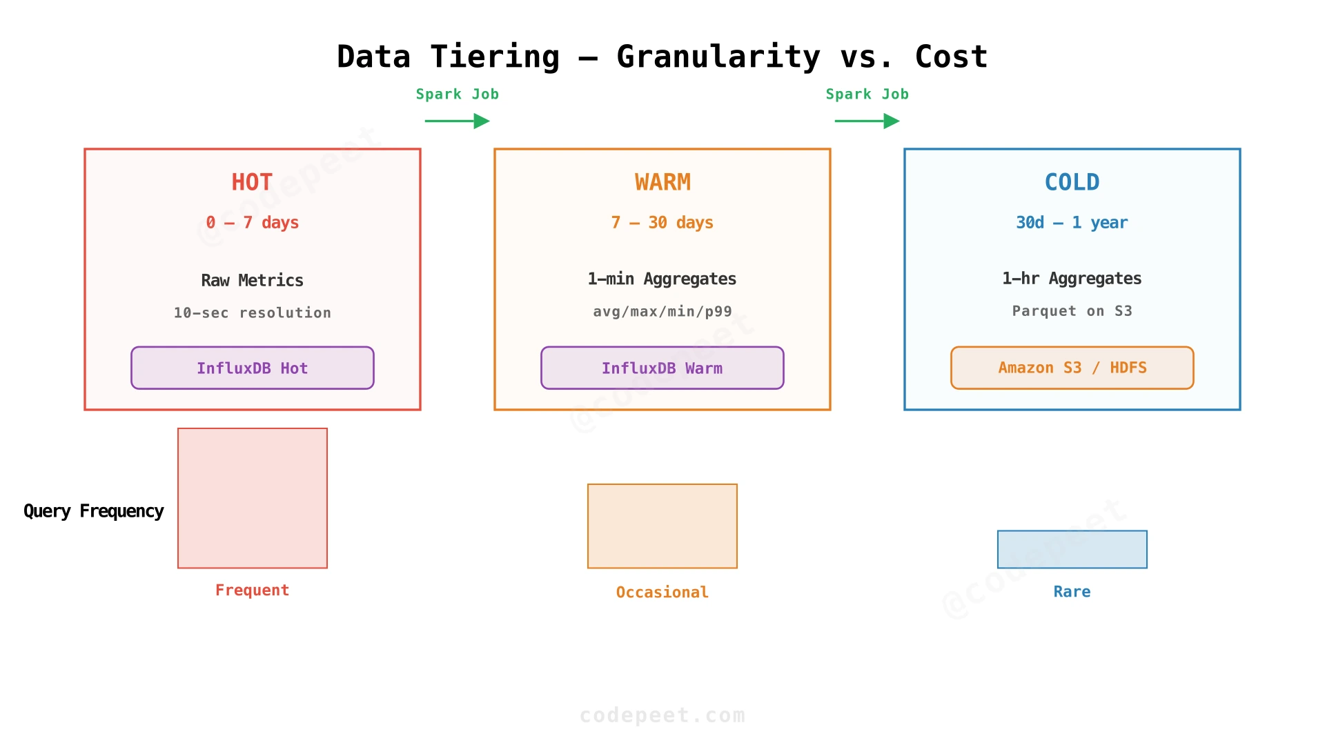
Monitoring data follows a clear access pattern: recent data is hot, old data is cold. We implement a three-tier storage strategy:
| Tier | Retention | Granularity | Storage | Query Speed |
|---|---|---|---|---|
| Hot | 0–7 days | Raw (10-sec resolution) | TSDB (InfluxDB) | < 100ms |
| Warm | 7–30 days | 1-minute aggregates | TSDB (separate retention policy) | < 500ms |
| Cold | 30 days–1 year | 1-hour aggregates | S3/HDFS + query engine | 1–5 sec |
The Batch Aggregator (Apache Spark job, runs hourly) handles the transitions:
- Read raw data older than 7 days from TSDB.
- Compute 1-minute aggregates (avg, max, min, p99 for each metric).
- Write aggregates to the warm tier (or a separate InfluxDB retention policy).
- The TSDB's built-in retention policy automatically drops raw data older than 7 days.
- After 30 days, another Spark job downsamples 1-minute data to 1-hour aggregates and archives to S3.
Cost comparison:
- InfluxDB Cloud: ~$1.44/GB/month
- Amazon S3 Standard: ~$0.023/GB/month
- Ratio: 63:1 — moving cold data to S3 cuts storage costs by 98%.
Deep Dives
Stream Processing and the Alert Engine
The alert engine is the most latency-sensitive component in the system. When a server's CPU spikes to 95%, the on-call engineer must be paged within 60 seconds — not after the data has been persisted to the TSDB and a batch job runs.
Why stream processing (not batch)?
If we evaluate alert rules by periodically querying the TSDB (e.g., every 30 seconds), we face two problems:
- Increased read pressure: Every alert rule generates a query. With hundreds of rules, we're hammering the TSDB with reads while it's already handling 6K writes/sec.
- Latency floor: The fastest alert delivery = rule_check_interval + query_time + notification_delivery. At 30-second polling, worst case is 30s + query_time + delivery.
With stream processing, the alert engine evaluates rules as data flows through Kafka, before it even reaches the TSDB. Alert latency is reduced to: Kafka_consumer_lag + rule_evaluation_time + notification_delivery ≈ seconds.
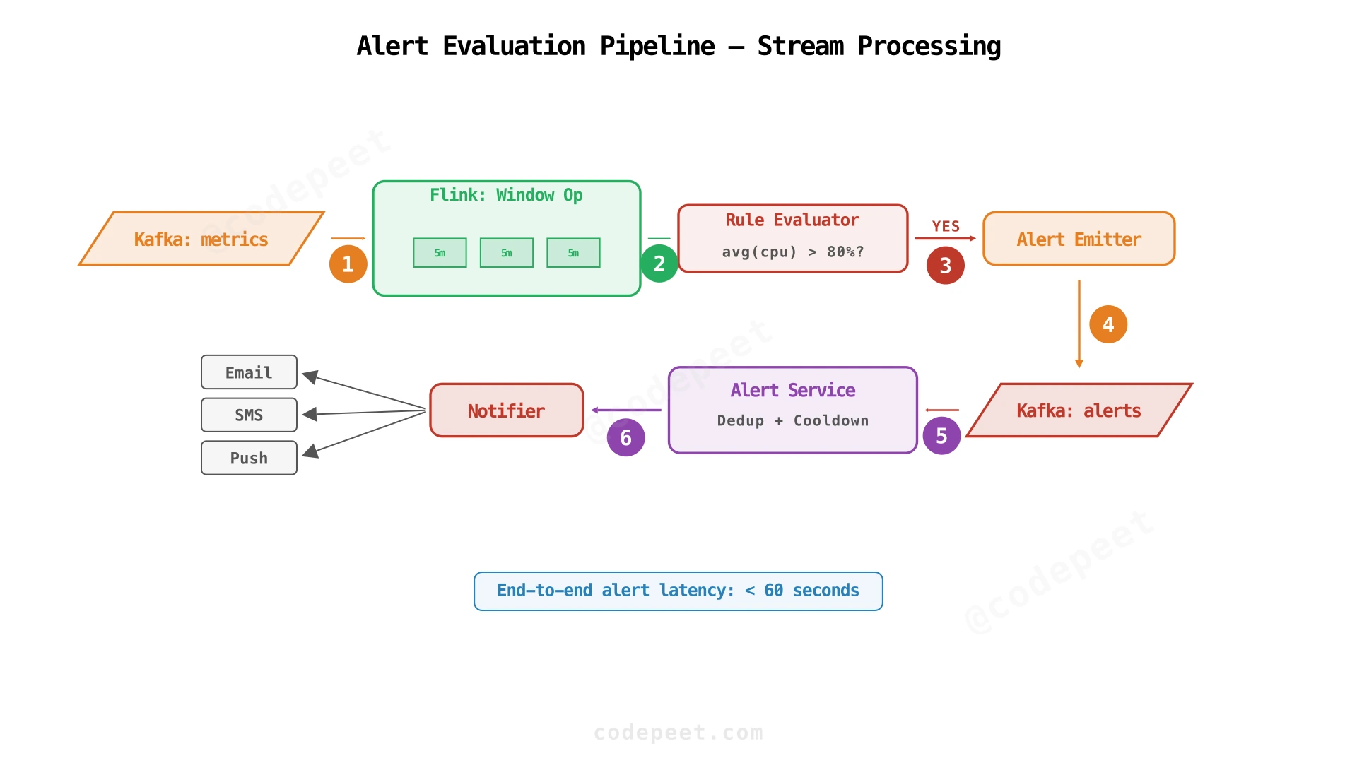
How Flink evaluates windowed alert rules:
Consider the rule: "Alert if avg CPU > 80% over 5 minutes for any production server."
- Keyed Stream: Flink keys the Kafka consumer by
server_id, ensuring all metrics from a single server are processed by the same Flink task. - Tumbling Window: A 5-minute tumbling window collects all
cpu_usagevalues for each server. - Aggregation: At window close, Flink computes
avg(cpu_usage)for each server. - Rule Evaluation: The aggregated value is compared against the rule's threshold. If
avg > 80, an alert event is emitted. - Watermarks: Flink uses event-time watermarks (based on agent timestamps) to handle out-of-order and late-arriving data. A configurable "allowed lateness" (e.g., 30 seconds) lets Flink wait for stragglers before closing the window.
Raw alert events from Flink can be noisy — if CPU stays above 80% for an hour, Flink emits an alert event every 5 minutes (12 alerts). The Alert Service must:
- Deduplication: Group alerts by (rule_id, server_id). If an alert is already open for this combination, don't send another notification.
- Cooldown: After an alert triggers, suppress re-notifications for a configurable period (e.g., 15 minutes) unless severity escalates.
- Escalation: If an alert remains open for N minutes without acknowledgment, escalate to the next level (e.g., from team Slack to on-call SMS to VP email).
- Resolution: When the metric drops below the threshold for a full window period, the alert is automatically resolved and a "resolved" notification is sent.
State for deduplication and cooldown is stored in Redis (fast lookups by composite key) with TTL-based expiration.
Production monitoring systems support several rule types:
| Rule Type | Example | Flink Implementation |
|---|---|---|
| Threshold | avg(cpu) > 80% over 5m | Tumbling window + aggregate + compare |
| Rate of change | disk_usage increased by 20% in 1h | Sliding window + delta calculation |
| Absence | No metrics received for 2 minutes | Session window with gap detection |
| Composite | cpu > 80% AND memory > 90% | Multi-stream join on server_id + window |
| Anomaly | CPU deviates > 3σ from 7-day average | Requires historical baseline from TSDB |
Threshold, rate-of-change, and absence rules can all be evaluated purely in the stream. Anomaly rules require enrichment from the TSDB (fetching baseline statistics), which adds latency but is still faster than polling.
Data Granularity vs. Aggregation — Hot/Warm/Cold Tiering
Monitoring data has a unique temporal value curve: the most recent data is queried constantly (dashboards showing the last hour), yesterday's data is occasionally queried (incident investigation), and last month's data is rarely accessed (capacity planning). Storing everything at raw granularity forever is both expensive and inefficient.
The fundamental trade-off: Higher granularity gives more detail for debugging but costs more to store and query. Lower granularity saves storage but loses the ability to see short-lived spikes.
Implementation: Downsampling pipeline
A Spark batch job runs hourly with the following logic:
- Raw → 1-minute: For data older than 7 days, group by
(server_id, metric, minute)and computeavg,max,min,p99,count. - 1-minute → 1-hour: For aggregated data older than 30 days, further aggregate to hourly granularity.
- Archive: Write 1-hour aggregates to S3 in Parquet format (columnar, compressed, queryable via Athena/Presto).
- Cleanup: TSDB's built-in retention policy drops raw data after 7 days and 1-minute data after 30 days automatically — no manual DELETE queries.
Aggregation functions preserved at each tier:
| Aggregation | Purpose | Example query |
|---|---|---|
avg | Typical value over window | "What was avg CPU last week?" |
max | Peak detection | "What was the highest memory usage yesterday?" |
min | Baseline detection | "What's the floor for disk I/O?" |
p99 | Tail latency / outlier detection | "What's the 99th percentile response time?" |
count | Volume estimation | "How many data points in this window?" |
By storing all five aggregations, we preserve enough statistical information to answer most queries without needing the raw data.
An optimization: instead of writing every raw metric directly to the TSDB, the TSDB Writer consumer can perform in-memory pre-aggregation over a short window (e.g., 10 seconds):
- Collect all metrics arriving in a 10-second micro-batch.
- If multiple data points exist for the same (server_id, metric) within the window, aggregate them (e.g., take the latest value, or compute avg).
- Write the single aggregated value to the TSDB.
This can reduce TSDB write volume significantly if agents send metrics more frequently than the 10-second interval (e.g., sub-second application metrics), or if there's jitter causing multiple points to arrive in the same window.
With 10K servers and 6 metrics, the micro-batch holds at most 60K entries — easily fits in memory (< 10 MB with overhead).
The monitoring agent can also aggregate locally before sending:
- Metric batching: Instead of sending one metric at a time, the agent collects all 6 metrics and sends them in a single payload. This is already our design.
- Local pre-aggregation: For high-frequency metrics (e.g., per-request latency measured 1000 times/sec), the agent computes 10-second histograms and sends only the summary (avg, p50, p99, max, count) instead of 10,000 raw values.
- Delta compression: For slowly-changing metrics (disk_usage), the agent can send only the delta from the last reported value, reducing payload size.
However, be cautious: aggressive client-side aggregation can hide short-lived spikes that a 10-second average would smooth out.
Scaling the System — 10× to 1000×
Our baseline: 10K servers, 6K writes/sec, 60 reads/sec. Let's examine how the system scales as the server fleet grows.
10× (100K servers, 60K writes/sec, 600 reads/sec)
- Kafka: Add partitions and brokers. Kafka scales linearly — 60K writes/sec is routine for a 6-broker cluster.
- Stream Processor: Add Flink task managers. Flink's parallel operators scale with Kafka partition count.
- TSDB: Single InfluxDB node handles ~100K field writes/sec. With 360K fields/sec (60K × 6 metrics), we need a 4-node InfluxDB cluster. TimescaleDB with multi-node is another option.
- Collector: Stateless — add more instances behind a load balancer.
- Dashboard API: Add replicas, introduce a caching layer (Redis) for repeated queries.
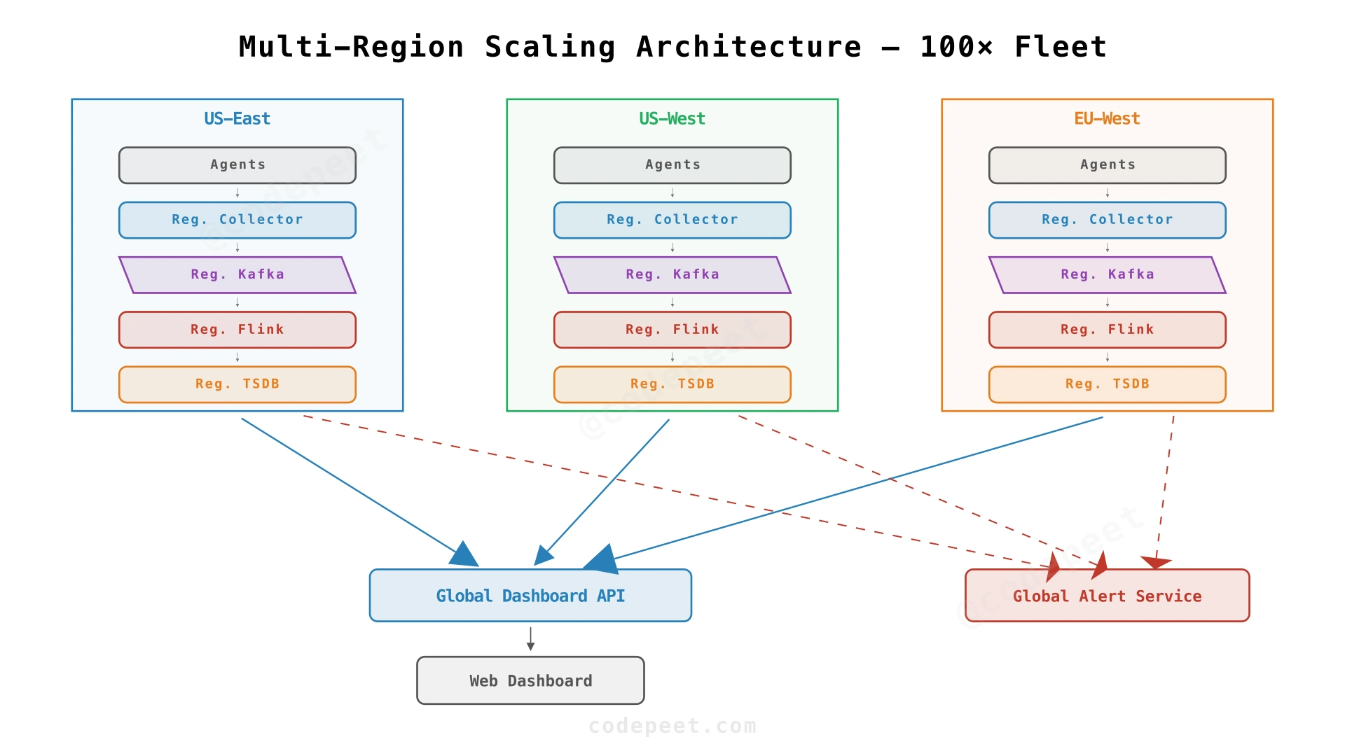
100× (1M servers, 600K writes/sec, 6K reads/sec)
- Kafka: 12–24 broker cluster with hundreds of partitions. Need dedicated hardware with SSDs for low-latency commits.
- TSDB: Must shard across 20+ nodes. Consider InfluxDB Enterprise or switch to VictoriaMetrics (designed for millions of time series).
- Stream Processor: 50+ Flink task slots. Alert rule count may also grow — need broadcast state pattern for rule distribution.
- Multi-region: Deploy regional ingestion clusters. Each region has its own Kafka + Flink + TSDB. A central dashboard aggregates across regions.
1000× (10M servers, 6M writes/sec, 60K reads/sec)
- This is Datadog/New Relic scale. Now you're building a SaaS platform.
- Multi-tenant isolation: Separate Kafka topics and TSDB databases per customer.
- Hierarchical aggregation: Agents report to regional collectors → regional TSDB → global aggregation service.
- Custom TSDB: At this scale, companies like Datadog build proprietary storage engines optimized for their access patterns.
- Cost optimization becomes paramount: Every byte per metric matters when you have 6 billion writes/sec.
Dashboard reads can spike when an incident triggers — all engineers load the dashboard simultaneously ("thundering herd" on reads). Strategies:
- Query result caching (Redis): Cache the results of common queries (e.g., "last 1 hour CPU for server X") with a short TTL (30 seconds). Since monitoring data for a past time window is immutable, cache invalidation is time-based, not event-based.
- Read replicas: Route dashboard queries to TSDB read replicas, keeping the primary for writes.
- Pre-computed materialized views: For standard dashboard panels (e.g., "avg CPU across all production servers"), pre-compute the values using Flink and store in a fast K/V store.
- Query fan-out: For cross-server aggregation queries, the Dashboard API can query multiple TSDB shards in parallel and merge results.
Dashboard Architecture and Real-Time Updates
The dashboard is the primary interface for engineers — it must render live metric graphs, support drill-down per server, and display alert status. The key challenge is delivering real-time updates without overwhelming the backend.
Polling vs. WebSocket vs. Server-Sent Events (SSE):
| Approach | Mechanism | Latency | Scalability | Use case |
|---|---|---|---|---|
| Polling | Client GETs /metrics every N seconds | Bounded by interval | Low server cost per client | Historical views |
| WebSocket | Bidirectional persistent connection | Near real-time | Higher server cost (stateful) | Live dashboards |
| SSE | Server pushes over HTTP | Near real-time | Moderate | Live dashboards (unidirectional) |
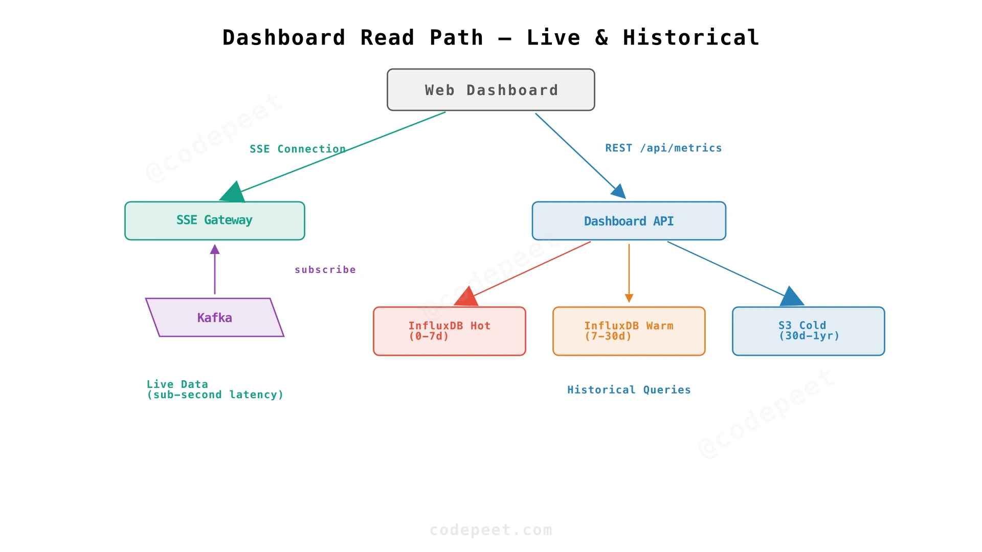
Recommendation: Hybrid. Use SSE for live dashboard panels (server pushes new data points as they arrive via Kafka → SSE gateway). Use REST polling for historical queries. This avoids the complexity of WebSocket connection management while still providing live updates.
The SSE Gateway is a separate service that:
- Subscribes to Kafka's
server_metricstopic (using a dedicated consumer group). - Maintains a mapping of active SSE connections → which server_ids/metrics each client is subscribed to.
- When a new metric arrives from Kafka, checks which SSE clients are interested and pushes the data point to them.
This avoids the dashboard needing to query the TSDB for live data. The dashboard receives data with sub-second latency after the agent sends it.
For historical data, the dashboard sends REST queries to the Dashboard API, which routes to the appropriate TSDB tier.
In practice, many teams use off-the-shelf visualization tools:
Grafana — The most popular open-source dashboarding tool. Connects to InfluxDB, TimescaleDB, Prometheus, and dozens of other data sources. Provides rich graphing, alerting, and annotation capabilities. Highly extensible with plugins.
Kibana — Best for log-centric monitoring (pairs with Elasticsearch). Excellent for full-text log search and visualization. Less optimal for pure metric dashboards.
Chronograf — InfluxData's companion tool. Tightly integrated with InfluxDB but narrower ecosystem than Grafana.
For an interview, mention that you'd use Grafana in production but the underlying architecture (how data gets to the dashboard) is what matters. Building a custom dashboard is rarely justified when Grafana exists.
Staff-Level Discussion Topics
These open-ended topics have no single correct answer — they test architectural judgment and the ability to reason about complex trade-offs. Use the discussion buttons to practice articulating your thinking.
If your monitoring system goes down during a production incident, you're flying blind. This creates a circular dependency: the tool that detects failures is itself a system that can fail. Staff candidates should discuss:
- Running a separate, minimal Prometheus instance that monitors only the monitoring pipeline itself.
- Heartbeat-based health checks: each component publishes a heartbeat — if a heartbeat is missed, a simple dead man's switch alerts via a completely independent channel (e.g., PagerDuty direct integration).
- Avoiding shared infrastructure between the primary monitoring pipeline and the self-monitoring pipeline.
- What metrics about the monitoring system matter: Kafka consumer lag, Flink checkpoint latency, TSDB write error rate, alert delivery success rate.
Evolving from an internal monitoring tool to a multi-tenant SaaS platform (like Datadog) introduces entirely new architectural concerns:
- Tenant isolation: Should each tenant get dedicated Kafka topics and TSDB databases, or share infrastructure with logical separation?
- Noisy neighbor: One customer sending 100× expected data volume could impact others. How do you implement per-tenant rate limiting without losing their data?
- Billing: Charge by metrics volume (data points/month), active time series, or queries? Each pricing model has different engineering implications.
- Data residency: EU customers may require their monitoring data to stay in EU regions.
Static threshold alerts (CPU > 80%) generate noise because the "normal" baseline varies: a server running a batch job at 3 AM might legitimately hit 95% CPU, while a web server at 50% during off-peak could be anomalous. Staff candidates should discuss:
- Statistical baselines: Compute per-server, per-metric, per-time-of-day baselines using historical data (e.g., 7-day rolling average with day-of-week seasonality).
- Z-score alerting: Alert when the current value deviates more than Nσ from the baseline.
- ML models: Train lightweight anomaly detection models (Isolation Forest, LSTM) on historical patterns and deploy them as Flink operators.
- Cold start problem: New servers have no baseline — how do you handle the first 7 days?
- Feedback loops: Allow engineers to mark alerts as false positives, feeding back into model training.
Level Expectations
What interviewers expect at each seniority level for a real-time monitoring system design:
| Area | |||
|---|---|---|---|
| Requirements | Lists FRs (collect, store, alert, dashboard) and basic NFRs (scale, latency) | Derives FRs systematically from verbs; quantifies NFRs with numbers (6K writes/sec, 60 reads/sec) | Identifies subtle NFRs: monitoring system must be more reliable than the systems it monitors; discusses self-monitoring |
| API Design | Defines /metrics ingest endpoint with JSON body | Explains async ingestion (202 Accepted), batch payloads, and idempotency | Discusses API versioning, agent backward compatibility, and graceful degradation |
| Architecture | Agent → Kafka → DB → Dashboard pipeline | Explains why each component exists (Kafka for durability + fan-out, Flink for real-time rules, TSDB for time-range queries) | Discusses push vs. pull trade-offs, evaluates Prometheus vs. push pipeline, and designs multi-region topology |
| Storage | Knows to use a TSDB | Explains TSDB advantages over RDBMS; designs schema with tags vs. fields; describes retention policies | Designs full tiered storage (hot/warm/cold), cost analysis (TSDB vs S3 at 63:1 ratio), and downsampling pipeline |
| Alerting | Rules are "checked against the database" | Explains stream processing for real-time evaluation; windowed aggregations | Designs complete alert lifecycle: dedup, cooldown, escalation, resolution; discusses composite and anomaly-based rules |
| Scaling | "Add more servers" | Explains Kafka partition scaling, TSDB sharding, read replicas | Designs 100×–1000× scaling strategy; discusses multi-region, hierarchical aggregation, custom TSDB at Datadog scale |
| Dashboard | "A web UI that shows graphs" | Explains REST for historical, SSE/WebSocket for live; caching for repeated queries | Designs SSE gateway architecture, pre-computed materialized views, thundering herd mitigation |
Interview Cheatsheet
Quick-reference talking points for the interview:
"A real-time monitoring system collects metrics from a server fleet, processes them through a streaming pipeline, stores them in a time-series database, evaluates alert rules in real-time, and serves dashboards for live and historical views. The key insight is that this is fundamentally a streaming data pipeline, not a request-response system."
- FRs: Collect (server metrics), Store (time-series), Alert (rule-based, < 1 min), Visualize (live + historical dashboard)
- NFRs: 10K servers → 6K writes/sec, 60 reads/sec, 99.99% availability, < 30s ingest-to-dashboard latency
- Out of scope: Log aggregation, distributed tracing, anomaly detection ML
- Agent (lightweight daemon on each server) — push model, batched every 10 seconds
- Collector/MQ Proxy (stateless HTTP) — validates and publishes to Kafka
- Kafka (message queue) — durability, peak absorption, fan-out to multiple consumers
- Flink (stream processor) — real-time alert rule evaluation on windowed data
- InfluxDB (TSDB) — time-series storage with built-in retention and downsampling
- Alert Service — dedup, cooldown, escalation, multi-channel notification
- Dashboard API + SSE Gateway — REST for historical, SSE for live updates
- Spark (batch aggregator) — downsample hot→warm→cold tiered storage
- Push vs. Pull: Push for real-time + firewall friendliness; Pull (Prometheus) for K8s service discovery
- Kafka before TSDB: Absorbs peaks, provides durability, enables stream processing fan-out
- TSDB vs. RDBMS: TSDB gives 10–50× better write throughput and compression for time-series data
- Stream vs. Batch alerting: Stream gives seconds latency; batch adds 30s+ per polling interval
- Data granularity vs. cost: Hot/warm/cold tiering with 63:1 cost ratio (TSDB vs S3)
- SSE vs. WebSocket: SSE is simpler for unidirectional live dashboard updates
| Metric | Value |
|---|---|
| Servers monitored | 10,000 (20% annual growth) |
| Metrics per server | 6 (CPU, memory, disk, net in, net out, app counter) |
| Collection interval | 10 seconds |
| Writes/sec | 6,000 steady, 18,000 peak |
| Reads/sec | 60 |
| Daily data volume | ~48 GB raw |
| Monthly raw | ~1.44 TB |
| Alert latency target | < 60 seconds end-to-end |
| TSDB vs S3 cost | 63:1 per GB |
- "How would you handle agent failures?" — Heartbeat monitoring: if agent misses 3 consecutive check-ins, the system generates an "agent down" alert. The collector tracks expected agents.
- "What about multi-tenant SaaS?" — Separate Kafka topics and TSDB organizations per tenant; rate limiting per tenant; billing based on metrics volume.
- "How would you add log aggregation?" — Similar pipeline: agent ships logs → Kafka → Elasticsearch (for full-text search) → Kibana. Logs and metrics share the Kafka backbone.
- "How do you monitor the monitoring system?" — Self-monitoring: internal health metrics published to a separate, minimal Prometheus instance. If the main pipeline goes down, the self-monitoring system alerts.