topk
Introduction
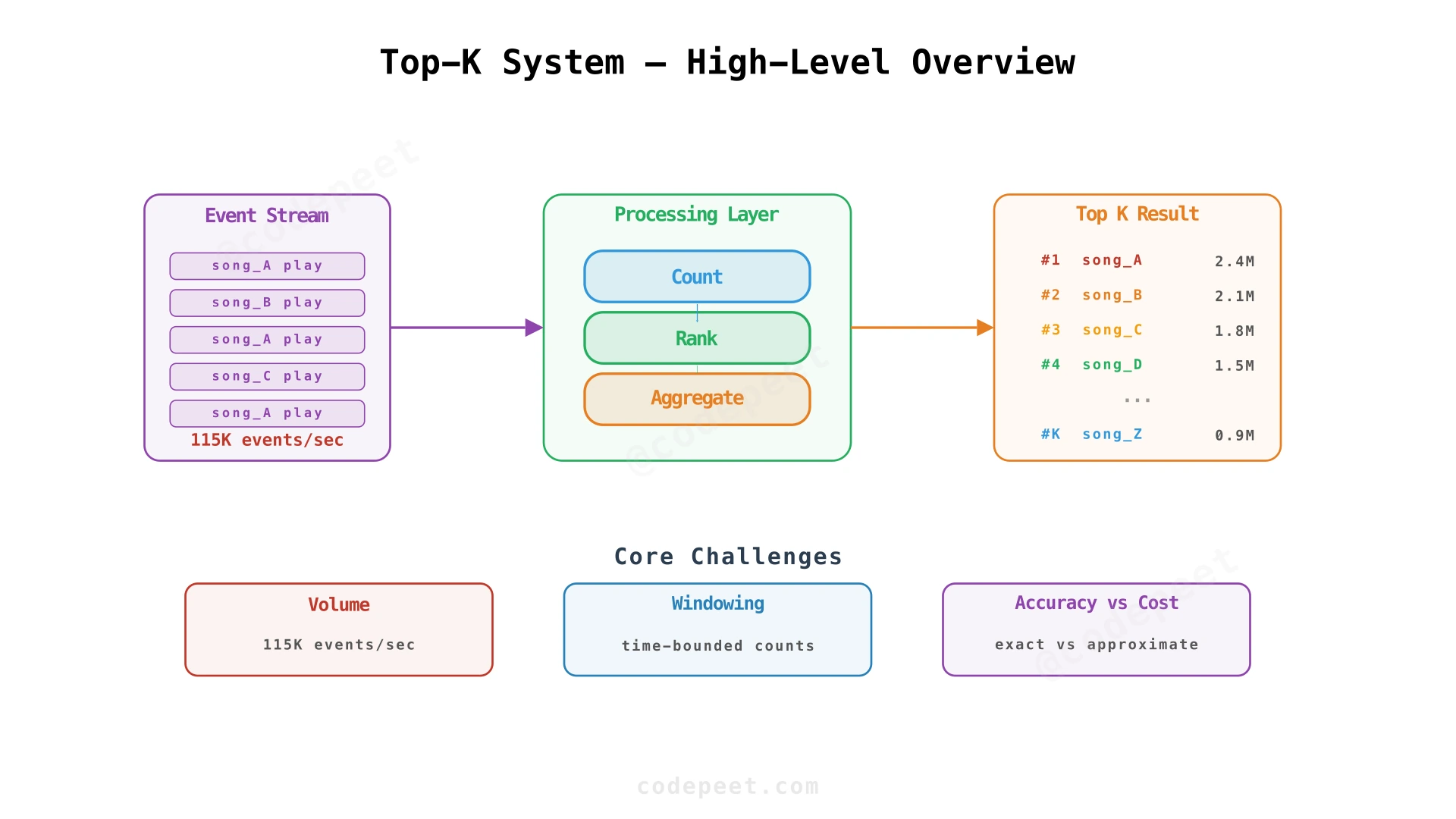
Top-K (also called "Heavy Hitters") is a foundational stream processing problem: given a continuous, high-volume stream of events, find the K most frequent items. We'll use Spotify's most-played songs as the running example — every song play is an event and we want the top K songs — but the same pattern applies to Amazon's trending products, YouTube's most-watched videos, Twitter's trending topics, and ad-click leaderboards.
It sounds like a straightforward aggregation query, but building it as a real-time system introduces several hard problems:
-
Volume — 10 billion song plays per day means ~115,000 events/second. A single machine can't count them all in memory. The system must partition work across many nodes while producing a single, correct top-K result.
-
Windowing — "Top songs of all time" is trivial to define but rarely what users want. Spotify's Top Songs playlist is the top songs today. That means the system must maintain time-windowed counts — and efficiently expire old events as they slide out of the window.
-
Accuracy vs Cost — Maintaining exact counts for 100 million distinct songs at 115K events/sec is expensive. In practice, approximate top-K (using probabilistic data structures like Count-Min Sketch) is often good enough. The system should support both exact and approximate modes.
The core tension is between freshness (results should reflect recent plays) and cost (counting everything exactly is expensive). A well-designed Top-K system lets you trade accuracy for throughput along a smooth spectrum.
At scale: 10B events/day, 100M distinct songs, top-K API accessed 1M times/day, K typically 100–1,000.
Functional Requirements
Unlike most system design problems where we extract multiple verbs, Top-K has a single core requirement — find the most frequent items — but it comes in progressively harder variants:
-
Global Top-K (Low QPS) — Users can view the top K most played songs of all time. Traffic is low enough that a single instance handles it. This is the "data structures" version of the problem.
-
Global Top-K (High QPS) — Same all-time top-K, but now traffic is 115K events/sec — far beyond a single instance. This forces us to partition and aggregate.
-
Sliding Window Top-K — Users can view the top K most played songs in the last X time (e.g., last 24 hours, last hour). This introduces event expiration and windowed counting.
Each variant builds on the previous one, forming a natural progressive architecture.
Out of Scope
- Ingesting streaming data (assumed to arrive via Kafka/Kinesis)
- User interface
- Exact ranking within the top K (order among the top items is approximate)
- Multi-tenancy (per-user top-K)
Non-Functional Requirements
We extract adjectives and descriptive phrases to identify quality constraints:
- "real-time" → Results must reflect recent data, not stale aggregations
- "accurate" → Top-K must be correct (or approximately correct with known error bounds)
- "scalable" → Must handle 10B events/day without degradation
- "fault-tolerant" → Crash recovery without replaying the entire stream
| NFR | Target | Reasoning |
|---|---|---|
| Low Latency | Top-K query response <100ms | Users expect instant leaderboard results — the top-K API is a read-heavy, latency-sensitive endpoint |
| High Throughput | 115K events/sec ingestion | 10B plays/day must be counted without event loss or backpressure on producers |
| Accuracy | Exact or bounded approximate (configurable) | Exact when K is small and data fits in memory; approximate (Count-Min Sketch) when memory or throughput constraints require it |
| Fault Tolerance | Crash recovery in <1 minute | If a counting node crashes, it must recover from a snapshot + replay a small offset window — not the entire stream |
| Freshness | Results reflect plays from the last few seconds | Stale results (showing yesterday's top songs) make the feature useless for trending content |
| Scalability | Horizontal scaling of counting nodes | Adding more partitions should linearly increase throughput |
Key insight: The fundamental trade-off in Top-K is accuracy vs throughput vs memory. Exact counting requires more memory (a hash map entry per distinct song). Approximate counting (Count-Min Sketch) uses fixed memory but introduces bounded error. The system should let operators choose where to sit on this spectrum.
Resource Estimation
Scale Assumptions
| Parameter | Value |
|---|---|
| Song plays per day | 10 billion |
| Distinct songs | 100 million |
| Top-K API requests per day | 1 million |
| K (top items returned) | 100–1,000 |
| Average event size | ~100 bytes (song_id + timestamp + metadata) |
| Sliding window duration | 1 hour to 24 hours |
Throughput
Event ingestion rate:
This is the key number — ~115K events/sec must be counted and ranked.
Top-K query QPS:
Read QPS is trivial. The challenge is entirely on the write (counting) side.
Memory
Exact counting (hash map per distinct song):
Each hash map entry: ~32 bytes (8B song_id hash + 8B count + 16B overhead)
This fits on a single large instance but leaves little room for the sliding window state. With partitioning across N nodes:
Min-heap for top-K:
The heap itself is negligible. The cost is in the full counting state.
Count-Min Sketch (approximate):
A sketch with error rate and failure probability :
For (0.1% error) and (99% confidence):
That's 109 KB vs 3.2 GB — a ~30,000× reduction. This is why approximate counting is so attractive at scale.
Bandwidth
Inbound (event stream):
Outbound (top-K API responses):
Bandwidth is not a bottleneck. The system is CPU and memory bound (counting operations and heap maintenance).
API Design
Top-K has a minimal API surface — one read endpoint. The complexity is entirely in the backend processing pipeline.
# ── Query Top-K Items ─────────────────────────────────────────
GET /api/top-items?k=100&time_window=1d
→ 200 OK
{
  "items": [
    { "id": "song_abc", "count": 2450000 },
    { "id": "song_def", "count": 2340000 },
    { "id": "song_ghi", "count": 2280000 }
  ],
  "window": { "type": "sliding", "duration": "24h" },
  "approximate": false,
  "generated_at": "2024-03-15T10:00:00Z"
}

# Parameters:
#   k            — number of top items to return (default: 100)
#   time_window  — time window for counts (e.g., 1h, 1d, all)
#                  defaults to 'all' (global window / all time)
Design Decisions
time_windowparameter — Supportsall(global/all-time), or a duration like1h,1d,7d. This maps to different backend processing pipelines (global window vs. sliding window).approximatefield in response — The response indicates whether the result is exact or approximate. This is transparent to the client — they can decide whether to display a disclaimer.- Pre-computed, not on-demand — The API reads from a pre-computed result cache, not by running a query over the event stream. The top-K is maintained continuously by the processing pipeline.
Background: Window Types
Before diving into the design, it's important to understand the three main windowing strategies used in stream processing:
Global Window — Covers all data from the beginning of time. All events land in one window. Use case: "top K songs of all time".
Timeline:      0     5    10    15    20    25    30
Events:        e1    e2   e3    e4    e5    e6    e7
Global Win: [---------------------------------------]
Tumbling Window — Fixed-size, non-overlapping windows. Events belong to exactly one window. Use case: "top K songs per hour" (each hour is independent).
Timeline:     0    5    10   15   20   25   30
Events:       e1   e2   e3   e4   e5   e6   e7
Tumbling Win: [----W1----][----W2----][---W3---]
Sliding Window — Fixed-size window that slides forward continuously. Events can belong to multiple overlapping windows. Use case: "top K songs in the last 24 hours" (updated continuously).
Timeline:      0    5    10   15   20   25   30
Events:        e1   e2   e3   e4   e5   e6   e7
Sliding Win: [----W1----]
                [----W2----]
                    [----W3----]
In production, Spotify's Top Songs is updated every 24 hours (a tumbling window). But for interview depth, we design for the harder sliding window variant — if you can solve sliding, tumbling is a trivial simplification.
High-Level Design
We build the architecture progressively, starting from a single-instance data structure problem and evolving through four iterations. Each step addresses a limitation that the previous design can't handle.
Step 1: Global Top-K on a Single Instance — Min-Heap + HashMap
The Starting Architecture
Start with the simplest case: one machine counts all song plays and maintains the top K. This is fundamentally a data structures problem.
The Data Structure: Min-Heap + HashMap
If you've solved LeetCode's "Top K Frequent Elements", the approach is familiar: a min-heap of size K keeps the K highest-count songs. The song at the root has the lowest count among the top K — any new song that exceeds this threshold displaces it.
Alongside the heap, a hash map stores two things per song:
- The total play count
- The song's index in the heap (if it's in the top K)
The heap index is critical for performance. When a song already in the top K gets another play, we need to update its count and re-heapify. Without the index, finding the song in the heap is O(K). With the index, it's O(1) lookup + O(log K) re-heapify.
class TopKTracker:
    def __init__(self, k):
        self.k = k
        self.heap = []            # min-heap of (count, song_id)
        self.counts = {}          # song_id -> total count
        self.heap_index = {}      # song_id -> index in heap

    def process_event(self, song_id):
        # Update count
        self.counts[song_id] = self.counts.get(song_id, 0) + 1
        count = self.counts[song_id]

        if song_id in self.heap_index:
            # Already in top-K: update count, bubble down
            idx = self.heap_index[song_id]
            self.heap[idx] = (count, song_id)
            self._sift_down(idx)
        elif len(self.heap) < self.k:
            # Heap not full: add directly
            self._push(count, song_id)
        elif count > self.heap[0][0]:
            # Beats the current minimum: replace root
            old_song = self.heap[0][1]
            del self.heap_index[old_song]
            self.heap[0] = (count, song_id)
            self.heap_index[song_id] = 0
            self._sift_down(0)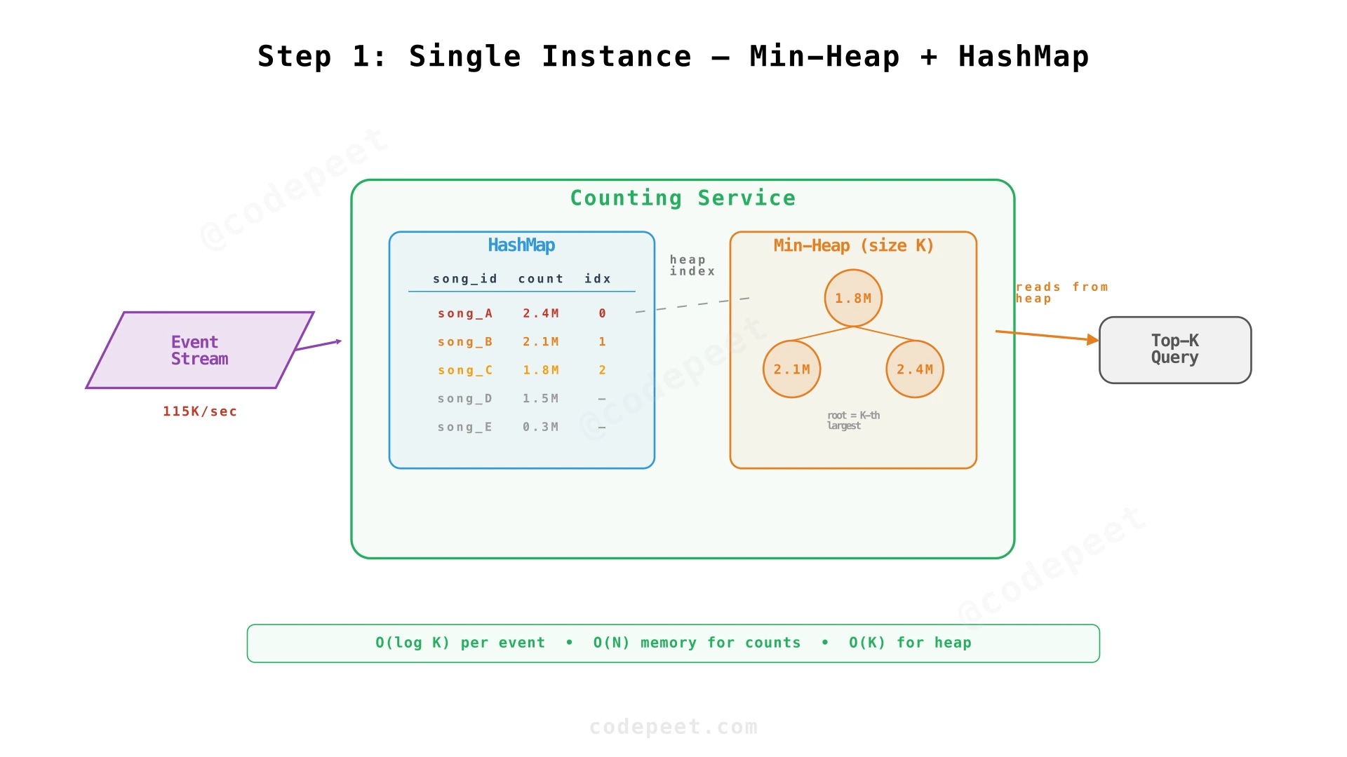
Complexity
| Operation | Time | Space |
|---|---|---|
| Process event (song already in top-K) | O(log K) | — |
| Process event (new song enters top-K) | O(log K) | — |
| Process event (no change to top-K) | O(1) | — |
| Query top-K | O(K log K) to sort | — |
| Total space | — | O(N) for counts + O(K) for heap |
Where N = number of distinct songs (100M) and K = top items (100–1,000).
✅ Works for: Low-throughput streams where one machine can handle all events. Correct, simple, and easy to implement.
❌ Missing: Can't handle 115K events/sec on a single machine. If the instance crashes, the in-memory heap and counts are lost. Only supports all-time (global window) counts.
Step 2: Partitioned Global Top-K — Hash Partitioning + Coordinator
Scaling Beyond a Single Machine
A single instance can't handle 115K events/sec. We need to partition the event stream across multiple counting nodes.
Partitioning Strategy
The key design decision: how do we route events to counting nodes?
| Strategy | How it works | Pros | Cons |
|---|---|---|---|
| Round-robin | Distribute events evenly | Even load | Same song counted on multiple nodes — requires merging all counts |
| Hash by song_id | partition = hash(song_id) % N | All plays for one song go to one node — clean per-partition top-K | Hot songs create hotspots |
| Consistent hashing | Song IDs mapped to a hash ring | Minimal rebalancing when nodes change | More complex setup |
We choose hash partitioning by song_id. Each counting node maintains a complete, correct count for its partition of songs. The coordinator doesn't need to merge raw counts — it only merges per-partition top-K results.
Coordinator Aggregation
Each partition maintains its own local top-K heap. A Coordinator Service periodically (or on query) collects the local top-K from each partition and merges them into a global top-K:
- Each of the N partitions returns its local top-K (K items)
- The Coordinator merges N × K items using a heap
- The final global top-K is the top K from the merged result
This works correctly because hash partitioning ensures a song's entire count lives on one partition. If song X is globally top-K, it must be in its partition's local top-K (assuming K is the same everywhere).
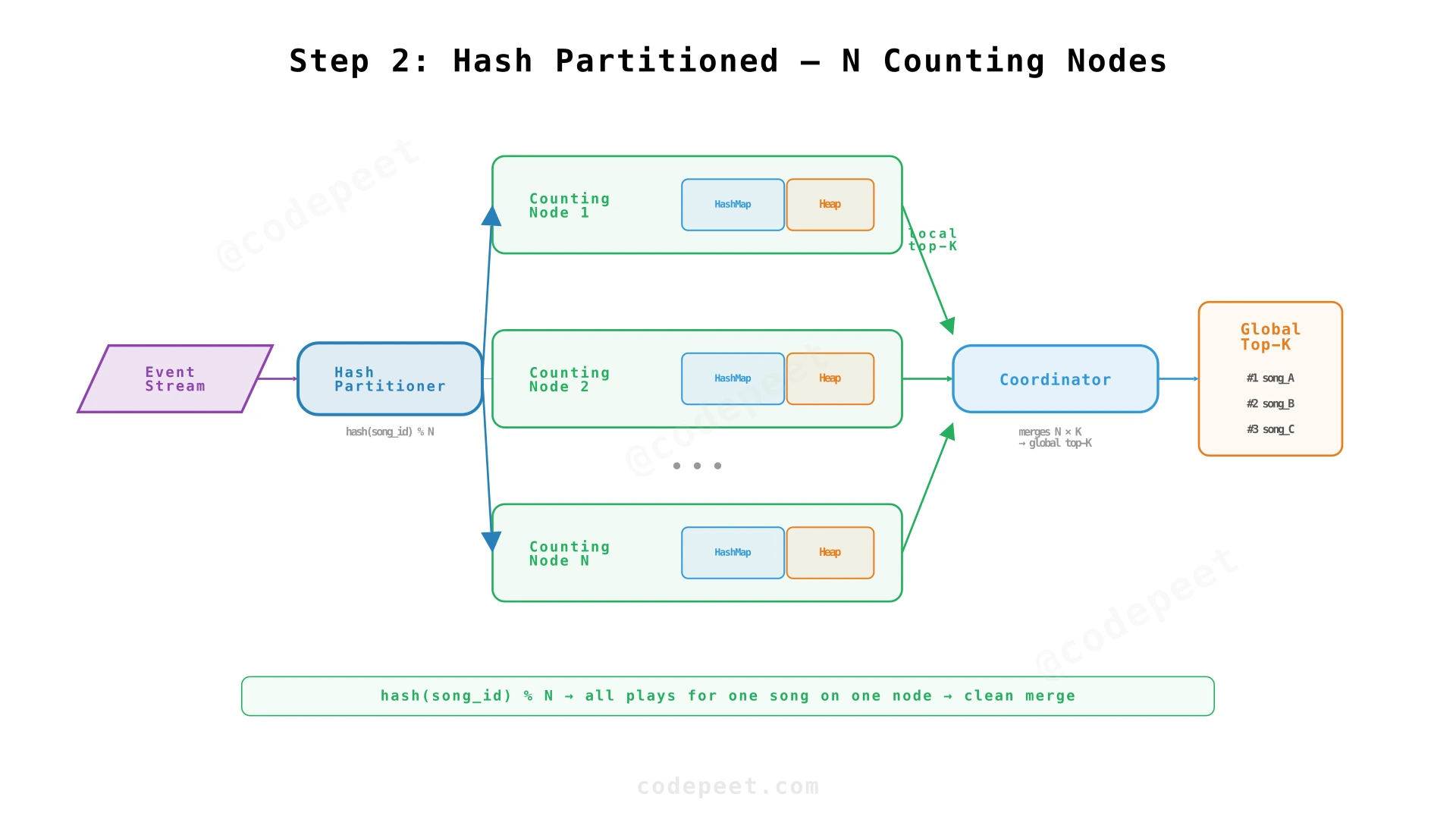
✅ NFRs addressed: Throughput (partitioned across N nodes — linear scaling), accuracy (hash partition ensures complete per-song counts)
❌ Still missing: If a counting node crashes, its in-memory state is lost. Recovery requires replaying the entire event stream from the beginning — too slow for a 10B events/day system. Still only supports global (all-time) window.
Step 3: Fault Tolerance — Snapshot + Stream Offset Recovery
Surviving Crashes Without Replaying Everything
If a counting node crashes, its heap and hash map are gone. Without persistence, recovery means replaying every event from the beginning of the stream — days or weeks of data. At 115K events/sec, even replaying one day takes ~24 hours at full speed. We need a smarter recovery strategy.
Periodic Snapshots
Each counting node periodically serializes its state to a durable store (S3, Redis, DynamoDB):
- Heap state — The current min-heap contents
- Count map — The full hash map of song_id → count
- Stream offset — The Kafka/Kinesis offset of the last event processed
On crash recovery:
- Load the latest snapshot → restores heap + counts to a known point
- Replay events only from the snapshot's stream offset to the current head
- The node is caught up after replaying a small window of events
Snapshot Interval Trade-off
- Frequent snapshots (every 1 min) → fast recovery, but more I/O and storage
- Infrequent snapshots (every 1 hour) → less overhead, but 1 hour of replay on recovery
A good default: snapshot every 5 minutes. At 115K events/sec, that's ~35M events to replay in the worst case — takes about 5 minutes at 2× ingestion speed.
Exactly-Once Semantics
The snapshot + offset approach gives us effectively exactly-once processing:
- Events before the snapshot offset are already counted (in the snapshot)
- Events after the snapshot offset are replayed on recovery
- The boundary is clean — no events are double-counted or missed
This is the same pattern used by Flink's checkpointing mechanism internally.
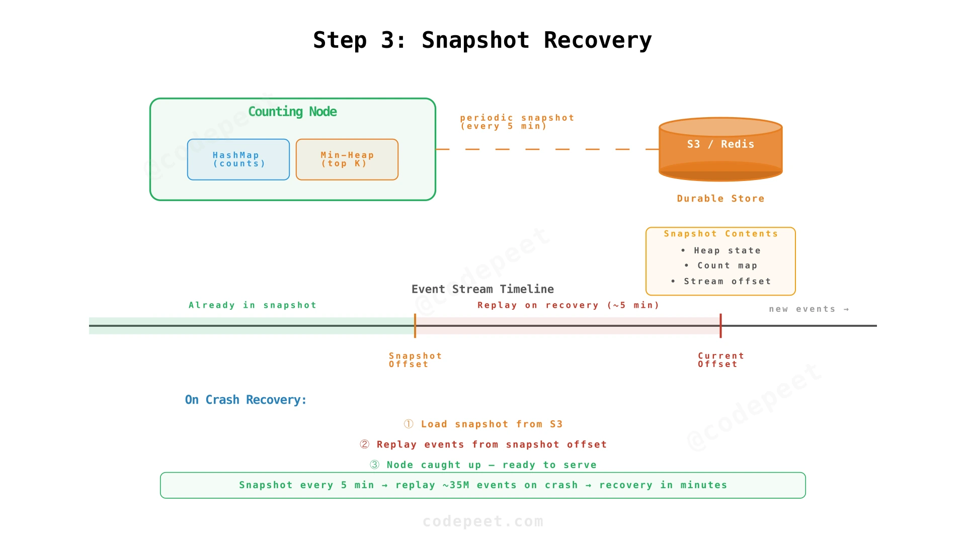
✅ NFRs addressed: Fault tolerance (crash recovery in minutes, not hours), data durability (state survives node failures)
❌ Still missing: Only supports global (all-time) window. Users asking "top songs in the last hour" can't be served — we'd need to expire old events and maintain time-bounded counts.
Step 4: Sliding Window Top-K — Dual-Offset Counting
Counting in a Moving Time Window
A sliding window requires two operations: adding new events as they arrive, and removing old events as they slide out of the window. Adding is easy — it's the same process_event logic. Removing is the hard part.
The Two-Pointer / Dual-Offset Approach
If you've solved sliding window problems on LeetCode, you know the two-pointer technique. We apply the same idea to stream offsets:
- End offset — Points to the latest event processed. Advances as new events arrive. Events at this offset are added to counts.
- Beginning offset — Points to the oldest event still within the window. Advances as time passes. Events at this offset are subtracted from counts.
The top-K result at any moment reflects only the events between the beginning and end offsets.
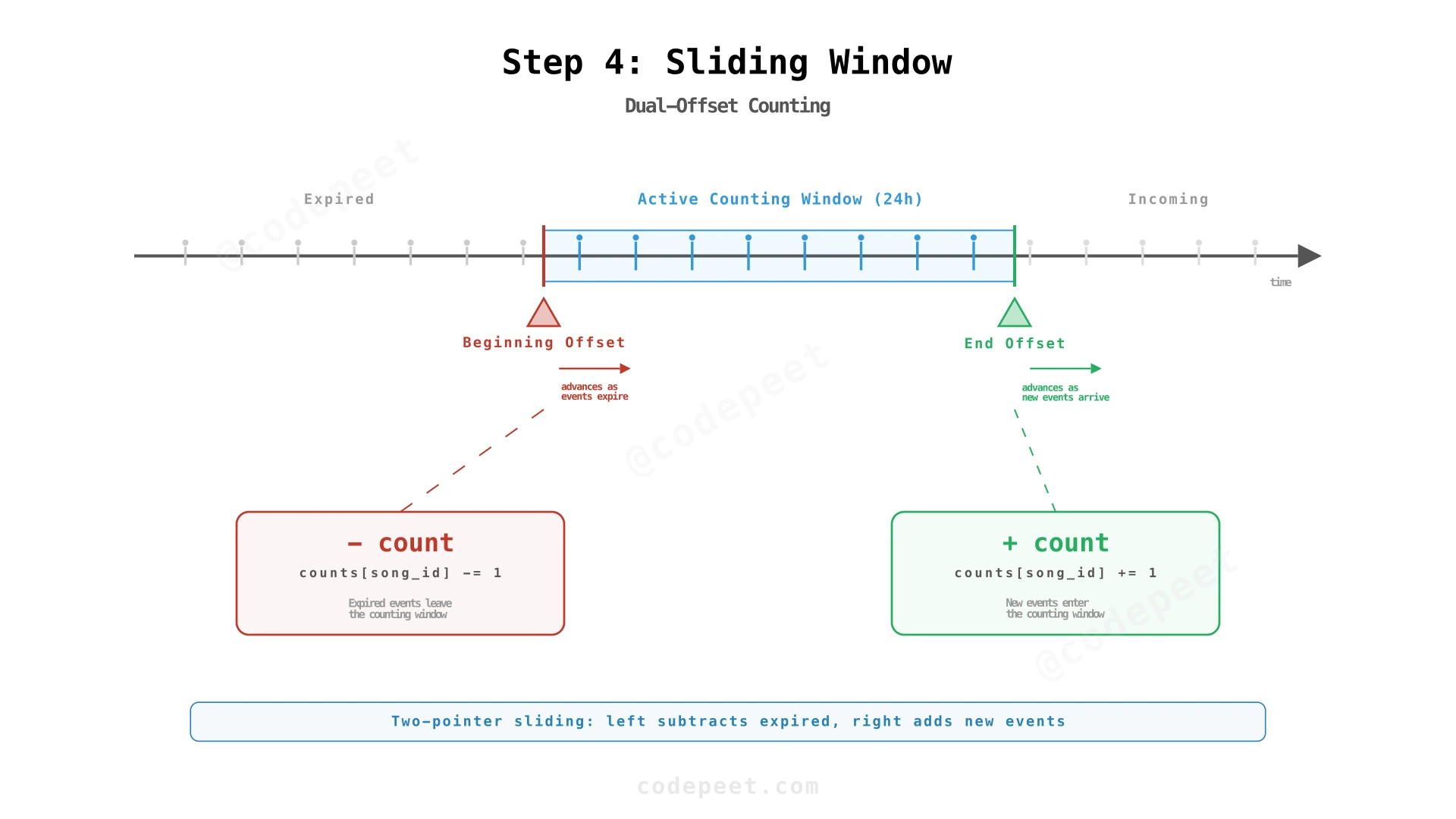
Processing Logic
For each window update cycle:
- Advance the end offset — Process new events using the standard heap logic (add to counts, update heap)
- Advance the beginning offset — For each expired event:
- Decrement the song's count in the hash map
- If the song is in the top-K heap and its count drops below the heap root, replace it
- If the count reaches zero, remove from the hash map
The Subtraction Problem
Removing events from a min-heap is harder than adding. When a song's count decreases, it might no longer deserve to be in the top-K. But which song replaces it? We'd need to scan all non-heap songs to find the new K-th largest — expensive.
Practical solution: Instead of maintaining a perfect top-K heap during subtraction, run a periodic recomputation. Every few seconds, rebuild the heap from the hash map (O(N) to find top K via selection algorithm). Between recomputations, the heap may be slightly stale — but for a music leaderboard, a few seconds of staleness is invisible to users.
Alternative: Bucketed Tumbling Windows
A simpler approximation: divide time into small tumbling buckets (e.g., 1-minute buckets). Each bucket stores its own count map. To answer "top-K in the last hour", aggregate the last 60 buckets. Old buckets are discarded entirely. This avoids per-event subtraction at the cost of bucket-boundary imprecision.
✅ NFRs addressed: Freshness (results reflect the current time window), query flexibility (any time window can be served)
❌ Still missing: At 115K events/sec with 100M distinct songs, exact counting requires ~3.2 GB of memory per window per partition. For multiple windows or limited memory, this is expensive.
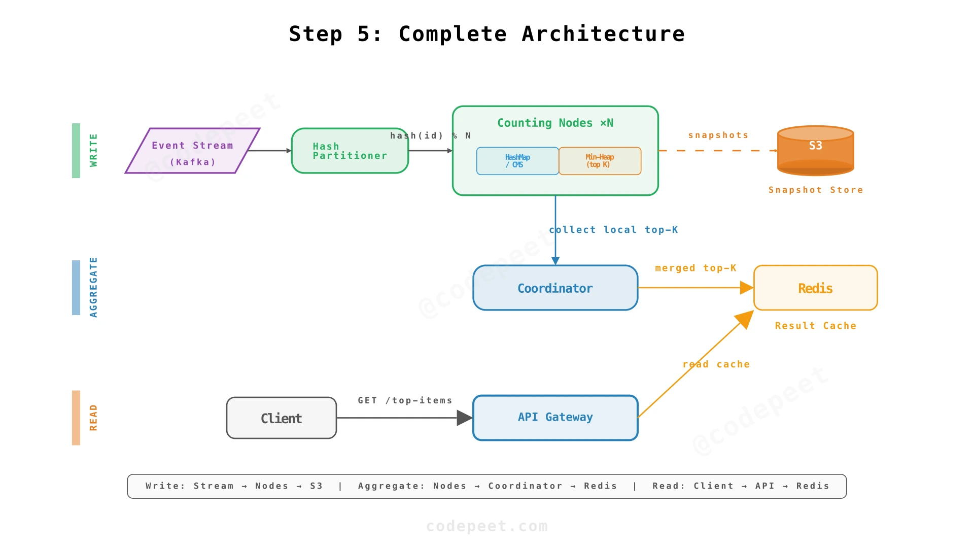
Step 5: Complete Architecture — Approximate Counting & Result Caching
The Final Architecture
The final pieces: approximate counting to reduce memory, and a result cache to serve the top-K API at low latency.
Count-Min Sketch for Approximate Counting
A Count-Min Sketch (CMS) is a probabilistic data structure that estimates frequencies using fixed memory. Instead of a hash map with one entry per distinct song, CMS uses a 2D array of counters with multiple hash functions:
- Structure:
depth × widthgrid of counters (e.g., 5 × 2,718 = ~109 KB) - Insert: Hash the song_id with each of the
depthhash functions, increment the corresponding counter in each row - Query: Hash the song_id, return the minimum across all rows (this minimizes overcounting from hash collisions)
CMS never undercounts — it can only overcount due to hash collisions. The error is bounded: with 99% probability, the overcount is at most 0.1% of total events.
When to use CMS vs exact counting:
| Scenario | Use Exact | Use CMS |
|---|---|---|
| K < 1,000, moderate cardinality | ✅ | — |
| K > 10,000 or very high cardinality | — | ✅ |
| Memory-constrained environments | — | ✅ |
| Legal/financial accuracy requirements | ✅ | — |
Result Cache
The top-K API doesn't query the counting nodes directly. Instead:
- The Coordinator periodically (every few seconds) collects local top-K from each partition
- Merges them into a global top-K
- Writes the result to a Redis cache or similar fast store
- The API Gateway reads from the cache — O(1) latency, no fan-out on read path
This separates the write path (event counting, high throughput) from the read path (top-K queries, low latency).
NFR Scorecard
| NFR | Target | How It's Met |
|---|---|---|
| Low Latency | <100ms query response | Pre-computed result in Redis cache; API reads from cache, not from counting nodes |
| High Throughput | 115K events/sec | Hash-partitioned across N counting nodes; each node processes its partition independently |
| Accuracy | Exact or bounded approximate | Exact mode: HashMap + Min-Heap. Approximate mode: Count-Min Sketch with configurable error bounds |
| Fault Tolerance | Recovery in <5 min | Periodic snapshots (heap + counts + stream offset) to durable storage; replay only from last snapshot |
| Freshness | Results within seconds of real-time | Coordinator polls counting nodes every few seconds; sliding window advances continuously |
| Scalability | Linear horizontal scaling | Add more partitions to increase throughput; Coordinator merge is O(N × K) — negligible |
Deep Dives
What if we only need approximate results?
Count-Min Sketch Deep Dive
If exact accuracy isn't required — and for most leaderboards it isn't — Count-Min Sketch (CMS) reduces memory by orders of magnitude while maintaining bounded error guarantees.
How CMS Works
CMS is a 2D array of counters with dimensions depth × width:
depth= number of independent hash functions (controls confidence)width= number of counters per hash function (controls accuracy)
Insert (song_id played):
for each hash function h_i (i = 1..depth):
    index = h_i(song_id) % width
    table[i][index] += 1
Query (how many plays for song_id?):
return min(table[i][h_i(song_id) % width] for i in 1..depth)
The minimum is taken because collisions can only increase a counter, never decrease it. The true count is always ≤ the CMS estimate.
Error Bounds
For a CMS with width and depth , and total events :
With and : the overcount is at most 0.04% of total events with 99.3% confidence.
CMS + Heap for Top-K
CMS alone only answers frequency queries — it doesn't track which items are most frequent. We combine CMS with a min-heap:
- On each event, update the CMS count for that song_id
- Query the CMS for the song's estimated count
- If the count exceeds the heap root, insert into the K-sized heap
This gives us approximate top-K in O(depth) time per event and O(width × depth + K) memory total.
CMS vs HashMap: When to Choose
| Dimension | HashMap | Count-Min Sketch |
|---|---|---|
| Memory | O(N) — one entry per distinct item | O(width × depth) — fixed, independent of N |
| Accuracy | Exact | Approximate (bounded overcount) |
| Insert | O(1) amortized | O(depth) |
| Deletion | O(1) | Not supported (for sliding window: use CMS per bucket) |
| Best for | Moderate cardinality, exact requirements | Very high cardinality, memory-constrained |
How do you handle hot keys in the partitioning scheme?
Hot Key Problem in Hash Partitioning
Hash partitioning routes all plays for a song to one node. But when a song goes viral (a new Taylor Swift release), that partition receives disproportionate traffic — potentially 10× the average — creating a hotspot.
Detecting Hot Keys
Before solving the problem, we need to detect it. Monitor per-partition event rates and flag partitions exceeding a threshold (e.g., 2× average). Alternatively, sample the event stream and run a small top-K on the sample to identify hot songs.
Strategies for Hot Keys
| Strategy | How it works | Tradeoff |
|---|---|---|
| Split hot partition | Sub-partition the hot key across M nodes, aggregate counts | More complex coordinator merge; needs to track which songs are split |
| Pre-aggregation layer | Add a combiner/pre-aggregation step before partitioning (like MapReduce's combiner) | Reduces per-node load but adds latency (batching) |
| Adaptive partitioning | Use consistent hashing with virtual nodes; hot partitions get more virtual nodes | Dynamic rebalancing; more infrastructure complexity |
| Accept skew + overprovision | Size each partition for 3-5× average load | Simple; wastes resources for non-hot partitions |
Pre-Aggregation (Recommended)
The most practical approach: add a combiner layer between the stream and the counting nodes. Multiple combiner instances accumulate counts for a short window (e.g., 1 second), then flush aggregated (song_id, delta_count) tuples to the counting nodes.
If a song gets 10,000 plays in one second across 10 combiners, each combiner sends one aggregated update (count: 1,000) instead of 1,000 individual events. The counting node sees 10 messages instead of 10,000 — a 1,000× reduction.
This is essentially the MapReduce combiner pattern applied to stream processing.
Sliding window vs tumbling window — when does the complexity pay off?
Window Strategy Analysis
An interviewer might challenge your window choice: "Do you really need a sliding window?" The answer depends on the product requirement.
Tumbling Window (Simpler)
- Fixed, non-overlapping time buckets (e.g., hourly)
- At each bucket boundary, reset all counts and start fresh
- No event subtraction needed — just discard old buckets
- Results change at bucket boundaries (potentially jarring for users)
Sliding Window (Smoother)
- Continuously moving window (e.g., "last 24 hours" always means the most recent 24h, not "since midnight")
- Requires event expiration (subtraction) as events leave the window
- Results update smoothly — no sudden resets
Hybrid: Bucketed Sliding Window
In practice, most production systems use a bucketed approximation of sliding windows:
- Divide time into small tumbling buckets (e.g., 1-minute buckets)
- Each bucket maintains its own count map
- To answer "top-K in the last hour": aggregate the last 60 buckets
- When a bucket expires (older than 1 hour), discard it entirely
This avoids per-event subtraction while giving results that are at most 1 bucket stale (1 minute in this example) — acceptable for virtually all leaderboard use cases.
Production Reality
- Spotify updates Top Songs daily (24-hour tumbling window)
- YouTube's Trending is updated hourly (1-hour tumbling)
- Twitter's Trending Topics use ~15-minute sliding windows
- Amazon's Best Sellers use daily tumbling windows
For most Top-K interviews, start with tumbling (show you understand the simple case), then propose sliding if the interviewer asks for more freshness.
How would you implement this using existing stream processing frameworks?
Production Implementation with Flink / Kafka Streams
In practice, you wouldn't build the counting and windowing infrastructure from scratch. Stream processing frameworks handle partitioning, windowing, fault tolerance, and exactly-once semantics out of the box.
Apache Flink Approach
Flink provides built-in windowing, state management, and checkpointing. A sliding window top-K in Flink is roughly:
// Flink sliding window top-K (simplified)
DataStream<Tuple2<String, Integer>> topK = songPlayStream
    .keyBy(event -> event.getSongId())    // partition by song
    .window(SlidingEventTimeWindows.of(
        Time.hours(24),           // window size
        Time.minutes(1)))         // slide interval
    .process(new TopKAggregator(K));  // custom aggregation
Flink handles:
- Partitioning:
.keyBy()does hash partitioning - Windowing:
.window()manages window boundaries and event assignment - Fault tolerance: Periodic checkpoints (snapshots) to durable storage
- Exactly-once: Via Chandy-Lamport distributed snapshot algorithm
Redis Sorted Set for Global Window
For the simpler global (all-time) top-K, a Redis sorted set (ZSET) is even simpler:
import redis
r = redis.Redis()

# On each song play:
r.zincrby('song_plays', 1, song_id)

# Query top-K:
top_songs = r.zrevrange('song_plays', 0, K - 1, withscores=True)
# Returns [(song_id, count), ...] sorted by count descending
Redis ZSET uses a skip list internally. ZINCRBY is O(log N) and ZREVRANGE is O(log N + K). For a global window with moderate cardinality, this is the simplest production-ready solution.
When to build from scratch vs use a framework:
| Scenario | Recommendation |
|---|---|
| Global window, moderate QPS | Redis ZSET |
| Sliding window, high QPS, exact | Flink/Spark Streaming |
| Sliding window, very high QPS, approximate | Custom CMS + heap |
| Interview | Design from scratch (shows understanding) |
<discuss-with-ai-button title="Production Stream Processing for Top-K" context="Flink provides built-in partitioning, windowing, and checkpointing. Redis ZSET is the simplest approach for global window top-K. In interviews, design from scratch to show understanding, then mention you'd use Flink in production." points='["How does Flink's checkpointing (Chandy-Lamport) compare to our manual snapshot approach?","What are the latency implications of using Flink vs a custom implementation?","How would you handle late-arriving events in Flink?","Can Redis ZSET handle 115K writes/sec — what are its limits?","How do you test a stream processing pipeline — can you simulate replay?"]'>
Staff-Level Discussion Topics
The following topics contain open-ended architectural questions for staff+ conversations.
Exactly-Once Processing in Distributed Stream Systems
Context: Our snapshot + offset approach gives effectively exactly-once processing within a single node. But in a distributed system with multiple partitions, a coordinator, and a result cache, end-to-end exactly-once is harder.
Discussion Points:
- The term "exactly-once" is controversial in distributed systems. What we actually achieve is "effectively exactly-once" — at-least-once delivery with idempotent processing.
- Flink achieves distributed exactly-once via the Chandy-Lamport distributed snapshot algorithm: all operators checkpoint their state simultaneously, with barrier markers flowing through the data stream to coordinate.
- Kafka Streams uses a transactional producer to atomically commit offsets and output records — tying consumption and production into a single transaction.
- For our custom system: what happens if the coordinator reads stale data from a partition during snapshot? Can we get an inconsistent global top-K?
- The practical question: does exact count matter for a leaderboard? If song A has 2,450,000 plays and song B has 2,449,999, does it matter which is #1?
<discuss-with-ai-button title="Exactly-Once in Distributed Streams" context="Exactly-once processing is achieved via snapshot + offset replay for single nodes. Distributed exactly-once uses Chandy-Lamport (Flink) or transactional commits (Kafka Streams). End-to-end exactly-once across the entire pipeline is challenging." points='["Is exactly-once processing truly achievable, or is it always effectively exactly-once with idempotent processing?","How does the Chandy-Lamport algorithm work in Flink — what are barrier markers?","What happens to exactly-once guarantees during coordinator failover?","Can you quantify the cost of exactly-once vs at-least-once — what's the throughput overhead?","Is exactly-once even worth the complexity for a leaderboard system?"]'>
Multi-Dimensional Top-K (Per-Region, Per-Genre, Per-User)
Context: Our design computes a single global top-K. But real products need multiple top-K views: top songs in the US, top songs in K-Pop genre, top songs for a specific user. How do you extend the system?
Discussion Points:
- Naive approach: Run a separate counting pipeline per dimension. 10 regions × 50 genres = 500 separate pipelines — doesn't scale.
- Pre-aggregation with dimensions: Each event carries dimensions
(song_id, region, genre, user_id). Counting nodes maintain per-dimension count maps. Memory cost: O(dimensions × distinct_songs). - Lambda architecture: Batch layer computes historical top-K per dimension (offline, MapReduce). Speed layer adds real-time deltas. Merge layer combines them for the query.
- OLAP approach: Write all events to a columnar store (ClickHouse, Druid) with dimensions as columns. Run GROUP BY + ORDER BY + LIMIT queries for arbitrary top-K slices. This trades real-time freshness for query flexibility.
- Per-user top-K is especially challenging: 10M users × 100M songs — can't pre-compute all combinations. Must use lazy evaluation or approximate user profiles.
Decay Functions: Time-Weighted Popularity
Context: A pure count-based top-K treats a play from 23 hours ago the same as a play from 1 minute ago. Real trending algorithms use decay — recent events count more than old ones. How do you incorporate time-weighted scoring?
Discussion Points:
- Exponential decay: Each event's weight decays as where is the age of the event and controls the decay rate. A song with 1,000 plays in the last hour scores higher than one with 10,000 plays spread over 24 hours.
- Implementation challenge: You can't just store a count — you need to store the decayed sum, which depends on the time of each event. Exact decay requires per-event timestamps.
- Approximation: Instead of exact decay, use bucketed weights. Plays in the last hour get weight 1.0, plays 1-6 hours ago get 0.5, plays 6-24 hours ago get 0.2. This maps to the bucketed tumbling window approach.
- Twitter's trending algorithm: Uses a combination of velocity (how fast counts are increasing) and volume, with exponential decay. A topic that suddenly spikes ranks higher than one with consistently high volume.
- Trade-off: Decay adds complexity to the counting infrastructure. Is it worth it? For a "Top Songs" playlist, probably not. For "Trending Now", absolutely.
<discuss-with-ai-button title="Time-Weighted Decay for Trending" context="Pure count-based top-K doesn't capture recency. Exponential decay weights recent events more. In practice, bucketed weights approximate true decay — plays in the last hour count more than plays from 12 hours ago." points='["How do you implement exponential decay in a streaming system without storing every event timestamp?","What decay rate should you use for a 24-hour trending playlist vs a 1-hour trending list?","How does Twitter's trending algorithm balance velocity vs volume?","Can you combine CMS with decay — what data structure supports both approximate counting and decay?","How do you backtest a decay function — how do you know the right lambda?"]'>
Level Expectations
| Dimension | |||
|---|---|---|---|
| Data Structures | Know that a min-heap solves top-K. Implement the basic heap + hashmap approach. Calculate time complexity. | Explain why the hashmap stores heap indices (O(1) lookup instead of O(K) scan). Discuss when to use CMS vs exact counting. | Analyze CMS error bounds mathematically. Propose hybrid approaches: exact counting for hot keys + CMS for long tail. Discuss space-optimal sketch parameters. |
| Partitioning | Know that a single machine can't handle 115K events/sec. Propose partitioning by song_id. | Compare round-robin vs hash vs consistent hashing. Explain why hash-by-song_id avoids cross-partition count merging. Design the coordinator merge. | Analyze hot key skew and propose pre-aggregation (combiner pattern). Design adaptive repartitioning. Discuss consistent hashing rebalancing impact on counts. |
| Windowing | Understand the difference between global and sliding windows. | Implement the dual-offset sliding window approach. Propose bucketed sliding as a practical approximation. Handle event expiration. | Analyze bucketed vs true sliding window accuracy tradeoffs. Propose decay functions for trending. Discuss late-arriving events and watermark strategies. |
| Fault Tolerance | Mention that in-memory state needs persistence. | Design the snapshot + offset recovery mechanism. Calculate recovery time based on snapshot frequency. | Discuss end-to-end exactly-once across distributed partitions. Compare to Flink's Chandy-Lamport checkpointing. Analyze failure modes: split-brain coordinator, partial snapshots. |
| Production | Mention that Flink/Spark could solve this. | Describe how Flink's .keyBy().window() maps to the manual design. Know Redis ZSET for global top-K. | Propose Lambda architecture for mixed batch + real-time. Design multi-dimensional top-K (per-region, per-genre). Discuss OLAP vs streaming tradeoffs (ClickHouse/Druid). |
Interview Cheatsheet
Core Architecture in 60 Seconds
"A stream processing pipeline with three layers. Events arrive via Kafka at 115K/sec. A hash partitioner routes events by song_id to N counting nodes. Each node maintains a HashMap of counts and a min-heap of size K. A coordinator periodically merges local top-K results into a global top-K and writes it to a Redis cache. The API reads from the cache — sub-millisecond response."
"Sliding window uses dual offsets. Each counting node tracks two stream pointers: the end offset (adds new events) and the beginning offset (subtracts expired events). The window between them holds the current counts. In practice, bucketed tumbling windows approximate sliding windows well enough."
"Fault tolerance via periodic snapshots. Each counting node snapshots its heap, counts, and stream offset to durable storage every 5 minutes. On crash, load the snapshot and replay only the events since the snapshot offset."
"For approximate results, Count-Min Sketch. Reduces memory from 3.2 GB (HashMap for 100M songs) to ~109 KB (fixed-size sketch). Never undercounts, overcounts by at most 0.1% of total events with 99% confidence."
Key Trade-offs to Mention
| Trade-off | Option A | Option B | When to Choose |
|---|---|---|---|
| Counting | Exact (HashMap) | Approximate (CMS) | Exact when memory allows and K is small; CMS for very high cardinality or constrained memory |
| Windowing | Tumbling (fixed buckets) | Sliding (continuous) | Tumbling for daily leaderboards; sliding for "trending now" freshness |
| Partitioning | Hash by song_id | Round-robin | Hash for clean per-song counts; round-robin only with global aggregation |
| Coordinator | Periodic polling | On-demand | Periodic for consistent cache; on-demand adds latency to each query |
| Snapshot frequency | Every 1 min | Every 10 min | Frequent for fast recovery; infrequent for less I/O overhead |
| Hot key handling | Pre-aggregation layer | Split partition | Pre-aggregation is simpler; split for extreme skew |
| Result serving | Direct from counting nodes | Redis cache | Always cache — decouples read path from write path |
Common Mistakes to Avoid
- ❌ Starting with Flink/Spark without explaining the underlying data structures — the interviewer wants to see you design the heap + hashmap, not configure a framework
- ❌ Forgetting that the hashmap needs heap indices — without them, updating a song's count in the heap is O(K) instead of O(log K)
- ❌ Using a max-heap instead of a min-heap — max-heap requires scanning all elements to find the K-th largest; min-heap's root is the K-th largest
- ❌ Ignoring crash recovery — in-memory heaps are lost on restart; without snapshots, you'd replay the entire event history
- ❌ Proposing sliding windows without addressing event expiration — adding events is easy, the hard part is efficiently removing them
- ❌ Serving top-K queries directly from counting nodes — adds fan-out latency; pre-compute and cache the result