Evaluate Division
Description
You are given a set of equations between pairs of variables along with their numerical results, and a list of queries asking for the result of dividing one variable by another.
Formally, you receive:
equations[i] = [Ai, Bi]meaning the variableAidivided by the variableBiequalsvalues[i].- A list of
queries[j] = [Cj, Dj]where you must computeCj / Dj.
If a query involves a variable not present in any equation, or if no chain of equations connects the two variables, return -1.0 for that query.
The key insight is that division relationships are transitive: if you know a / b = 2 and b / c = 3, then a / c = (a / b) × (b / c) = 6. This transitivity means you can chain known ratios together to answer queries about variables that are not directly related by a single equation.
Also note that a / a = 1.0 for any known variable, and a / b = 1 / (b / a) — every relationship is bidirectional.
Examples
Example 1
Input: equations = [["a","b"],["b","c"]], values = [2.0, 3.0], queries = [["a","c"],["b","a"],["a","e"],["a","a"],["x","x"]]
Output: [6.00000, 0.50000, -1.00000, 1.00000, -1.00000]
Explanation:
- a / b = 2.0 and b / c = 3.0 are given.
- a / c = (a / b) × (b / c) = 2.0 × 3.0 = 6.0. We chain through b.
- b / a = 1 / (a / b) = 1 / 2.0 = 0.5. The inverse of a known equation.
- a / e = -1.0 because variable e does not appear in any equation.
- a / a = 1.0 because any variable divided by itself is 1.
- x / x = -1.0 because x is undefined — it never appears in the equations.
Example 2
Input: equations = [["a","b"],["b","c"],["bc","cd"]], values = [1.5, 2.5, 5.0], queries = [["a","c"],["c","b"],["bc","cd"],["cd","bc"]]
Output: [3.75000, 0.40000, 5.00000, 0.20000]
Explanation:
- a / c = (a / b) × (b / c) = 1.5 × 2.5 = 3.75.
- c / b = 1 / (b / c) = 1 / 2.5 = 0.4.
- bc / cd = 5.0 (directly given).
- cd / bc = 1 / (bc / cd) = 1 / 5.0 = 0.2.
Note that "bc" and "cd" are variable names (strings), not products of b×c or c×d.
Example 3
Input: equations = [["a","b"]], values = [0.5], queries = [["a","b"],["b","a"],["a","c"],["x","y"]]
Output: [0.50000, 2.00000, -1.00000, -1.00000]
Explanation:
- a / b = 0.5 (directly given).
- b / a = 1 / 0.5 = 2.0 (inverse).
- a / c = -1.0 (c is not in any equation — no path from a to c).
- x / y = -1.0 (neither x nor y appear in equations).
Constraints
- 1 ≤ equations.length ≤ 20
- equations[i].length == 2
- 1 ≤ Ai.length, Bi.length ≤ 5
- values.length == equations.length
- 0.0 < values[i] ≤ 20.0
- 1 ≤ queries.length ≤ 20
- queries[i].length == 2
- 1 ≤ Cj.length, Dj.length ≤ 5
- Ai, Bi, Cj, Dj consist of lowercase English letters and digits
- The input is always valid — no division by zero, no contradictions
Editorial
Brute Force
Intuition
The simplest way to think about this problem is to precompute the division result for every pair of variables that can be connected through the equations, and then answer each query with a direct lookup.
Imagine you have a table (like a multiplication table in school, but for division). The rows and columns are the variables (a, b, c, ...). Cell (i, j) holds the value of variable_i / variable_j. Initially, you only know a few cells (the directly given equations and their inverses). You then fill in the rest by chaining: if you know a/b and b/c, you can compute a/c.
This is essentially the Floyd-Warshall approach: for every intermediate variable k, and every pair (i, j), check if you can compute i/j by going through k. If ratio[i][k] and ratio[k][j] are both known, then ratio[i][j] = ratio[i][k] × ratio[k][j].
After running this triple loop, every answerable query is a simple table lookup.
Step-by-Step Explanation
Let's trace through with equations = [["a","b"],["b","c"]], values = [2.0, 3.0]:
Step 1: Collect all unique variables: {a, b, c}. Create a ratio table initialized to -1.0 for all pairs, except ratio[x][x] = 1.0 for every known variable.
Step 2: Fill in directly given equations and their inverses:
- ratio[a][b] = 2.0, ratio[b][a] = 1/2.0 = 0.5
- ratio[b][c] = 3.0, ratio[c][b] = 1/3.0 ≈ 0.333
Table so far:
| a | b | c | |
|---|---|---|---|
| a | 1.0 | 2.0 | -1.0 |
| b | 0.5 | 1.0 | 3.0 |
| c | -1.0 | 0.333 | 1.0 |
Step 3: Floyd-Warshall — try every variable k as an intermediate:
- k = a: Check all pairs (i, j). For (b, c): ratio[b][a] × ratio[a][c] — but ratio[a][c] is -1.0, so skip. For (c, b): ratio[c][a] × ratio[a][b] — ratio[c][a] is -1.0, skip. No new cells filled.
Step 4: k = b: Check all pairs (i, j).
- (a, c): ratio[a][b] × ratio[b][c] = 2.0 × 3.0 = 6.0. Fill ratio[a][c] = 6.0!
- (c, a): ratio[c][b] × ratio[b][a] = 0.333 × 0.5 = 0.1667. Fill ratio[c][a] = 0.1667!
Step 5: k = c: No new pairs to fill (all reachable pairs already computed).
Final table:
| a | b | c | |
|---|---|---|---|
| a | 1.0 | 2.0 | 6.0 |
| b | 0.5 | 1.0 | 3.0 |
| c | 0.1667 | 0.333 | 1.0 |
Step 6: Answer queries by table lookup:
- a/c → ratio[a][c] = 6.0
- b/a → ratio[b][a] = 0.5
Floyd-Warshall — Filling the Division Ratio Table — Watch how the ratio table is gradually filled using known equations and intermediate variables, until every reachable pair has a computed value.
Algorithm
- Collect all unique variables from equations. Assign each an index 0, 1, 2, ...
- Create a V×V ratio table initialized to -1.0. Set ratio[i][i] = 1.0 for all i.
- For each equation (A, B) with value v:
- Set ratio[A][B] = v and ratio[B][A] = 1.0 / v.
- Run Floyd-Warshall: for each intermediate variable k, for each pair (i, j):
- If ratio[i][k] ≥ 0 and ratio[k][j] ≥ 0 and ratio[i][j] < 0:
- Set ratio[i][j] = ratio[i][k] × ratio[k][j].
- If ratio[i][k] ≥ 0 and ratio[k][j] ≥ 0 and ratio[i][j] < 0:
- For each query (C, D):
- If C or D not in the variable set, return -1.0.
- Otherwise, return ratio[C][D].
Code
class Solution {
public:
    vector<double> calcEquation(vector<vector<string>>& equations, vector<double>& values, vector<vector<string>>& queries) {
        // Collect unique variables and assign indices
        unordered_map<string, int> idx;
        int id = 0;
        for (auto& eq : equations) {
            if (idx.find(eq[0]) == idx.end()) idx[eq[0]] = id++;
            if (idx.find(eq[1]) == idx.end()) idx[eq[1]] = id++;
        }
        int n = id;
        // Initialize ratio table
        vector<vector<double>> ratio(n, vector<double>(n, -1.0));
        for (int i = 0; i < n; i++) ratio[i][i] = 1.0;
        for (int i = 0; i < (int)equations.size(); i++) {
            int a = idx[equations[i][0]], b = idx[equations[i][1]];
            ratio[a][b] = values[i];
            ratio[b][a] = 1.0 / values[i];
        }
        // Floyd-Warshall
        for (int k = 0; k < n; k++)
            for (int i = 0; i < n; i++)
                for (int j = 0; j < n; j++)
                    if (ratio[i][k] > 0 && ratio[k][j] > 0 && ratio[i][j] < 0)
                        ratio[i][j] = ratio[i][k] * ratio[k][j];
        // Answer queries
        vector<double> result;
        for (auto& q : queries) {
            if (idx.find(q[0]) == idx.end() || idx.find(q[1]) == idx.end())
                result.push_back(-1.0);
            else
                result.push_back(ratio[idx[q[0]]][idx[q[1]]]);
        }
        return result;
    }
};
class Solution:
def calcEquation(self, equations: list[list[str]], values: list[float], queries: list[list[str]]) -> list[float]:
# Collect unique variables and assign indices
idx = {}
for a, b in equations:
if a not in idx:
idx[a] = len(idx)
if b not in idx:
idx[b] = len(idx)
n = len(idx)
# Initialize ratio table
ratio = [[-1.0] * n for _ in range(n)]
for i in range(n):
ratio[i][i] = 1.0
for i, (a, b) in enumerate(equations):
ia, ib = idx[a], idx[b]
ratio[ia][ib] = values[i]
ratio[ib][ia] = 1.0 / values[i]
# Floyd-Warshall
for k in range(n):
for i in range(n):
for j in range(n):
if ratio[i][k] > 0 and ratio[k][j] > 0 and ratio[i][j] < 0:
ratio[i][j] = ratio[i][k] * ratio[k][j]
# Answer queries
result = []
for c, d in queries:
if c not in idx or d not in idx:
result.append(-1.0)
else:
result.append(ratio[idx[c]][idx[d]])
return resultclass Solution {
public double[] calcEquation(List<List<String>> equations, double[] values, List<List<String>> queries) {
Map<String, Integer> idx = new HashMap<>();
int id = 0;
for (List<String> eq : equations) {
if (!idx.containsKey(eq.get(0))) idx.put(eq.get(0), id++);
if (!idx.containsKey(eq.get(1))) idx.put(eq.get(1), id++);
}
int n = id;
double[][] ratio = new double[n][n];
for (double[] row : ratio) Arrays.fill(row, -1.0);
for (int i = 0; i < n; i++) ratio[i][i] = 1.0;
for (int i = 0; i < equations.size(); i++) {
int a = idx.get(equations.get(i).get(0));
int b = idx.get(equations.get(i).get(1));
ratio[a][b] = values[i];
ratio[b][a] = 1.0 / values[i];
}
for (int k = 0; k < n; k++)
for (int i = 0; i < n; i++)
for (int j = 0; j < n; j++)
if (ratio[i][k] > 0 && ratio[k][j] > 0 && ratio[i][j] < 0)
ratio[i][j] = ratio[i][k] * ratio[k][j];
double[] result = new double[queries.size()];
for (int i = 0; i < queries.size(); i++) {
String c = queries.get(i).get(0), d = queries.get(i).get(1);
if (!idx.containsKey(c) || !idx.containsKey(d))
result[i] = -1.0;
else
result[i] = ratio[idx.get(c)][idx.get(d)];
}
return result;
}
}Complexity Analysis
Time Complexity: O(V³ + E + Q)
Where V is the number of unique variables, E is the number of equations, and Q is the number of queries. Floyd-Warshall runs in O(V³) for the triple nested loop. Building the initial table takes O(E). Each query is O(1) lookup after precomputation. With constraints V ≤ 40 and E ≤ 20, the V³ term is at most ~64,000 which is very fast.
Space Complexity: O(V²)
The ratio table is a V×V matrix. The variable-to-index map takes O(V) space. Total: O(V²).
Why This Approach Is Not Efficient
The Floyd-Warshall approach works well for this problem's constraints (V ≤ 40), but it has two conceptual inefficiencies:
-
O(V³) precomputation regardless of query count. If there are only a few queries, we might be computing far more ratios than we actually need. For example, with 40 variables but only 2 queries, we compute 1,600 ratios even though we only need 2.
-
O(V²) space for the full table. Every pair gets stored, even if most pairs are in disconnected components and will never be queried.
A better approach is to model this as a graph problem and only compute ratios on-demand per query. Each equation a/b = v creates a weighted edge from a to b (weight v) and from b to a (weight 1/v). To answer a query c/d, we simply find a path from c to d in this graph and multiply the edge weights along the path. This avoids precomputing unnecessary ratios and naturally handles disconnected components.
Better Approach - BFS on Weighted Graph
Intuition
Think of each variable as a city and each equation as a road with a conversion rate. The equation a/b = 2.0 means there is a road from city a to city b with a "conversion factor" of 2.0, and a road back from b to a with factor 0.5.
To answer the query a/c, we need to find a route from city a to city c and multiply all the conversion factors along the way. This is exactly a graph traversal problem!
We build a weighted directed graph where:
- Each variable is a node.
- Each equation a/b = v creates two edges: a→b with weight v, and b→a with weight 1/v.
For each query (C, D), we run a BFS (or DFS) from C. At each step, we track the accumulated product of edge weights from C. When we reach D, the accumulated product is our answer. If we exhaust all reachable nodes without finding D, the answer is -1.0.
This approach is more natural than Floyd-Warshall: we only do work when a query arrives, and we only explore the relevant connected component.
Step-by-Step Explanation
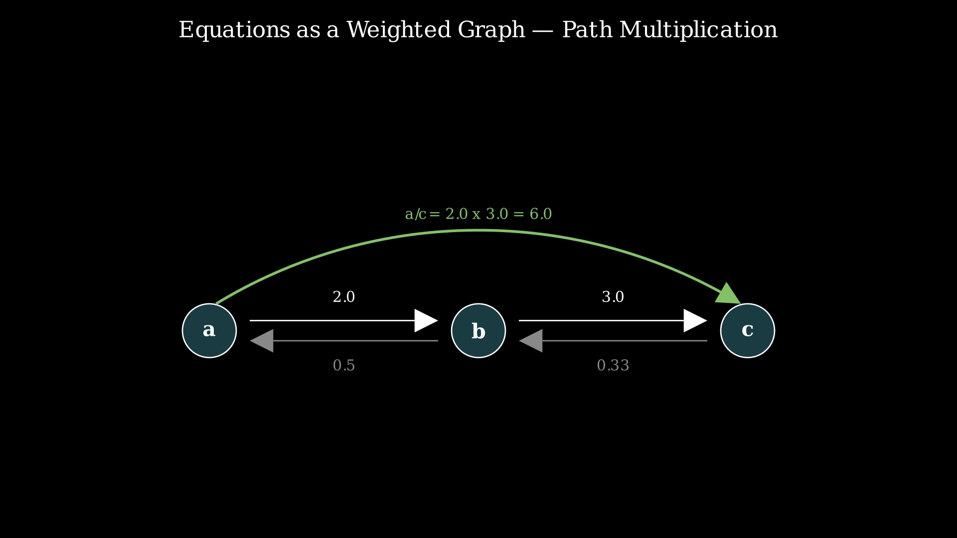
Let's trace through with equations = [["a","b"],["b","c"]], values = [2.0, 3.0], query = a / c:
Step 1: Build the graph. Each equation creates two directed edges:
- a → b (weight 2.0), b → a (weight 0.5)
- b → c (weight 3.0), c → b (weight 0.333)
Step 2: Process query a / c. Start BFS from node 'a' with accumulated product = 1.0.
Step 3: Initialize BFS queue with (a, 1.0). Mark 'a' as visited. Target is 'c'.
Step 4: Dequeue (a, 1.0). Check neighbors of 'a': only 'b' with edge weight 2.0. New product = 1.0 × 2.0 = 2.0. Is 'b' the target 'c'? No. Enqueue (b, 2.0). Mark 'b' as visited.
Step 5: Dequeue (b, 2.0). Check neighbors of 'b': 'a' (visited, skip) and 'c' with weight 3.0. New product = 2.0 × 3.0 = 6.0. Is 'c' the target? YES!
Step 6: Return 6.0. The path a → b → c gives product 2.0 × 3.0 = 6.0, which means a/c = 6.0.
For query b / a: BFS from 'b'. Neighbor 'a' with weight 0.5. Product = 1.0 × 0.5 = 0.5. Target reached. Return 0.5.
BFS on Weighted Graph — Finding a/c — Watch BFS traverse the weighted graph from node 'a' to node 'c', accumulating edge weight products along the path to compute a/c = 6.0.
Algorithm
- Build the graph: Create an adjacency list. For each equation (A, B) with value v:
- Add edge A → B with weight v.
- Add edge B → A with weight 1/v.
- Process each query (C, D):
a. If C or D is not in the graph, return -1.0.
b. If C == D, return 1.0.
c. Run BFS from C:- Initialize queue with (C, 1.0). Mark C as visited.
- While queue is not empty:
- Dequeue (node, product).
- For each neighbor (next, weight) of node:
- If next == D, return product × weight.
- If next not visited, mark visited, enqueue (next, product × weight).
- If BFS exhausts without finding D, return -1.0.
- Return all query results.
Code
class Solution {
public:
    vector<double> calcEquation(vector<vector<string>>& equations, vector<double>& values, vector<vector<string>>& queries) {
        // Build adjacency list
        unordered_map<string, vector<pair<string, double>>> graph;
        for (int i = 0; i < (int)equations.size(); i++) {
            string a = equations[i][0], b = equations[i][1];
            graph[a].push_back({b, values[i]});
            graph[b].push_back({a, 1.0 / values[i]});
        }

        vector<double> result;
        for (auto& q : queries) {
            string src = q[0], dst = q[1];
            if (graph.find(src) == graph.end() || graph.find(dst) == graph.end()) {
                result.push_back(-1.0);
                continue;
            }
            if (src == dst) {
                result.push_back(1.0);
                continue;
            }
            // BFS
            queue<pair<string, double>> bfs;
            unordered_set<string> visited;
            bfs.push({src, 1.0});
            visited.insert(src);
            double ans = -1.0;
            while (!bfs.empty()) {
                auto [node, prod] = bfs.front();
                bfs.pop();
                for (auto& [next, w] : graph[node]) {
                    if (next == dst) {
                        ans = prod * w;
                        break;
                    }
                    if (visited.find(next) == visited.end()) {
                        visited.insert(next);
                        bfs.push({next, prod * w});
                    }
                }
                if (ans > 0) break;
            }
            result.push_back(ans);
        }
        return result;
    }
};
from collections import defaultdict, deque
class Solution:
def calcEquation(self, equations: list[list[str]], values: list[float], queries: list[list[str]]) -> list[float]:
# Build adjacency list
graph = defaultdict(list)
for i, (a, b) in enumerate(equations):
graph[a].append((b, values[i]))
graph[b].append((a, 1.0 / values[i]))
def bfs(src: str, dst: str) -> float:
if src not in graph or dst not in graph:
return -1.0
if src == dst:
return 1.0
visited = {src}
queue = deque([(src, 1.0)])
while queue:
node, product = queue.popleft()
for neighbor, weight in graph[node]:
if neighbor == dst:
return product * weight
if neighbor not in visited:
visited.add(neighbor)
queue.append((neighbor, product * weight))
return -1.0
return [bfs(c, d) for c, d in queries]class Solution {
public double[] calcEquation(List<List<String>> equations, double[] values, List<List<String>> queries) {
Map<String, List<double[]>> graph = new HashMap<>();
Map<String, List<String>> neighbors = new HashMap<>();
for (int i = 0; i < equations.size(); i++) {
String a = equations.get(i).get(0), b = equations.get(i).get(1);
graph.computeIfAbsent(a, k -> new ArrayList<>()).add(new double[]{i, values[i]});
graph.computeIfAbsent(b, k -> new ArrayList<>()).add(new double[]{i, 1.0 / values[i]});
neighbors.computeIfAbsent(a, k -> new ArrayList<>()).add(b);
neighbors.computeIfAbsent(b, k -> new ArrayList<>()).add(a);
}
// Simplified adjacency using Map<String, Map<String, Double>>
Map<String, Map<String, Double>> adj = new HashMap<>();
for (int i = 0; i < equations.size(); i++) {
String a = equations.get(i).get(0), b = equations.get(i).get(1);
adj.computeIfAbsent(a, k -> new HashMap<>()).put(b, values[i]);
adj.computeIfAbsent(b, k -> new HashMap<>()).put(a, 1.0 / values[i]);
}
double[] result = new double[queries.size()];
for (int q = 0; q < queries.size(); q++) {
String src = queries.get(q).get(0), dst = queries.get(q).get(1);
if (!adj.containsKey(src) || !adj.containsKey(dst)) {
result[q] = -1.0;
continue;
}
if (src.equals(dst)) {
result[q] = 1.0;
continue;
}
// BFS
Queue<Object[]> bfs = new LinkedList<>();
Set<String> visited = new HashSet<>();
bfs.offer(new Object[]{src, 1.0});
visited.add(src);
double ans = -1.0;
while (!bfs.isEmpty()) {
Object[] curr = bfs.poll();
String node = (String) curr[0];
double prod = (double) curr[1];
for (Map.Entry<String, Double> entry : adj.get(node).entrySet()) {
String next = entry.getKey();
double w = entry.getValue();
if (next.equals(dst)) {
ans = prod * w;
break;
}
if (!visited.contains(next)) {
visited.add(next);
bfs.offer(new Object[]{next, prod * w});
}
}
if (ans > 0) break;
}
result[q] = ans;
}
return result;
}
}Complexity Analysis
Time Complexity: O(Q × (V + E))
Where Q is the number of queries, V is the number of unique variables, and E is the number of equations. For each query, BFS visits at most V nodes and E edges. Building the graph takes O(E). Total: O(E + Q × (V + E)).
With constraints (E ≤ 20, Q ≤ 20, V ≤ 40), this is at most ~20 × (40 + 20) = 1,200 operations per query — extremely fast.
Space Complexity: O(V + E)
The adjacency list stores V nodes and 2E directed edges (each equation creates two edges). The BFS visited set uses O(V) per query. Total: O(V + E).
Why This Approach Is Not Efficient
The BFS approach is already very efficient for this problem's constraints. However, it has one theoretical weakness: each query triggers a fresh BFS traversal. If there are many queries about the same connected component, we redo the graph traversal from scratch each time.
For problems with many queries (say Q = 10^5), this becomes O(Q × V) total, which could be slow.
A more elegant approach uses Union-Find (Disjoint Set Union) with weighted path compression. The idea is to preprocess all equations into a single data structure where each variable stores its ratio to its component's root. Then every query becomes a near-O(1) lookup: just divide the two variables' ratios to the root. This gives O(α(V)) per query after O(E × α(V)) preprocessing, where α is the inverse Ackermann function — effectively constant.
Optimal Approach - Weighted Union-Find
Intuition
Imagine each variable has a hidden "absolute value" that we do not know, but the equations tell us the ratios between them. For instance, a/b = 2 means a's value is exactly twice b's value. If we arbitrarily assign some variable (say the root of each component) a reference value of 1.0, we can compute every other variable's value relative to this root.
This is precisely what Weighted Union-Find does:
- Each variable starts as its own component with weight 1.0 (its ratio to itself).
- When we process equation a/b = v, we "union" their components. We maintain a weight
w[x]for every variable x such thatw[x] = x / root(x)— the ratio of x to the root of its component. - When we union the components of a and b, we compute the correct weight for connecting the two roots using the formula:
w[root_a] = v × w[b] / w[a]. - Path compression in
find()keeps chains short AND updates weights along the way by multiplying through the chain.
To answer query c/d:
- If c and d are in different components (or undefined): return -1.0.
- If same component: return
w[c] / w[d]— both are ratios to the same root, so their ratio gives c/d directly.
The beauty of this approach is that after preprocessing, every query is nearly O(1). No graph traversal needed.
Step-by-Step Explanation
Let's trace through with equations = [["a","b"],["b","c"]], values = [2.0, 3.0]:
Step 1: Initialize Union-Find. Each variable is its own parent with weight 1.0:
- parent = {a:a, b:b, c:c}
- weight = {a:1.0, b:1.0, c:1.0}
Step 2: Process equation a/b = 2.0. Find roots: find(a)=a, find(b)=b. Different roots, so union them. Make b the parent of a's root. Calculate weight: w[root_a] = v × w[b] / w[a] = 2.0 × 1.0 / 1.0 = 2.0.
- parent = {a:b, b:b, c:c}
- weight = {a:2.0, b:1.0, c:1.0}
- Meaning: a/b = w[a]/w[b] = 2.0/1.0 = 2.0 ✓
Step 3: Process equation b/c = 3.0. Find roots: find(b)=b, find(c)=c. Different roots, union them. w[root_b] = 3.0 × 1.0 / 1.0 = 3.0.
- parent = {a:b, b:c, c:c}
- weight = {a:2.0, b:3.0, c:1.0}
- Meaning: b/c = w[b]/w[c] = 3.0/1.0 = 3.0 ✓
Step 4: Query a/c. Call find(a):
- a's parent is b (not itself). Save origin = b. Recursively find(b).
- b's parent is c (not itself). Save origin = c. Recursively find(c) → returns c (root).
- Update w[b] = w[b] × w[origin_of_b] = 3.0 × 1.0 = 3.0. Set parent[b] = c.
- Back to a: update w[a] = w[a] × w[origin_of_a] = 2.0 × 3.0 = 6.0. Set parent[a] = c.
- After compression: parent = {a:c, b:c, c:c}, weight = {a:6.0, b:3.0, c:1.0}
Step 5: find(c) = c. Both a and c have root c.
- a/c = w[a] / w[c] = 6.0 / 1.0 = 6.0 ✓
Step 6: Query b/a. find(b) = c, find(a) = c. Same root.
- b/a = w[b] / w[a] = 3.0 / 6.0 = 0.5 ✓
Weighted Union-Find — Building and Querying Division Ratios — Watch how Union-Find maintains weight ratios to the root of each component. Path compression updates weights so that every query is a simple division of two weights.
Algorithm
- Initialize Union-Find: For each variable in equations, set
parent[x] = xandweight[x] = 1.0. - Define
find(x)with path compression:
a. If parent[x] ≠ x:- Save origin = parent[x].
- Recursively find root: parent[x] = find(parent[x]).
- Update weight: weight[x] *= weight[origin].
b. Return parent[x].
- Process each equation (A, B) with value v:
a. root_a = find(A), root_b = find(B).
b. If root_a == root_b, skip (already connected).
c. Union: parent[root_a] = root_b.
d. Weight: weight[root_a] = v × weight[B] / weight[A]. - Answer each query (C, D):
a. If C or D not in parent, return -1.0.
b. If find(C) ≠ find(D), return -1.0 (different components).
c. Otherwise return weight[C] / weight[D].
Code
class Solution {
public:
    unordered_map<string, string> parent;
    unordered_map<string, double> weight;

    string find(const string& x) {
        if (parent[x] != x) {
            string origin = parent[x];
            parent[x] = find(parent[x]);
            weight[x] *= weight[origin];
        }
        return parent[x];
    }

    vector<double> calcEquation(vector<vector<string>>& equations, vector<double>& values, vector<vector<string>>& queries) {
        // Initialize
        for (auto& eq : equations) {
            if (parent.find(eq[0]) == parent.end()) {
                parent[eq[0]] = eq[0];
                weight[eq[0]] = 1.0;
            }
            if (parent.find(eq[1]) == parent.end()) {
                parent[eq[1]] = eq[1];
                weight[eq[1]] = 1.0;
            }
        }
        // Union
        for (int i = 0; i < (int)equations.size(); i++) {
            string a = equations[i][0], b = equations[i][1];
            string ra = find(a), rb = find(b);
            if (ra == rb) continue;
            parent[ra] = rb;
            weight[ra] = values[i] * weight[b] / weight[a];
        }
        // Query
        vector<double> result;
        for (auto& q : queries) {
            string c = q[0], d = q[1];
            if (parent.find(c) == parent.end() || parent.find(d) == parent.end() || find(c) != find(d)) {
                result.push_back(-1.0);
            } else {
                result.push_back(weight[c] / weight[d]);
            }
        }
        return result;
    }
};
from collections import defaultdict
class Solution:
def calcEquation(self, equations: list[list[str]], values: list[float], queries: list[list[str]]) -> list[float]:
parent = {}
weight = defaultdict(lambda: 1.0)
def find(x: str) -> str:
if parent[x] != x:
origin = parent[x]
parent[x] = find(parent[x])
weight[x] *= weight[origin]
return parent[x]
# Initialize each variable as its own parent
for a, b in equations:
if a not in parent:
parent[a] = a
if b not in parent:
parent[b] = b
# Process equations (union)
for i, (a, b) in enumerate(equations):
ra, rb = find(a), find(b)
if ra == rb:
continue
parent[ra] = rb
weight[ra] = values[i] * weight[b] / weight[a]
# Answer queries
result = []
for c, d in queries:
if c not in parent or d not in parent or find(c) != find(d):
result.append(-1.0)
else:
result.append(weight[c] / weight[d])
return resultclass Solution {
Map<String, String> parent = new HashMap<>();
Map<String, Double> weight = new HashMap<>();
String find(String x) {
if (!parent.get(x).equals(x)) {
String origin = parent.get(x);
parent.put(x, find(parent.get(x)));
weight.put(x, weight.get(x) * weight.get(origin));
}
return parent.get(x);
}
public double[] calcEquation(List<List<String>> equations, double[] values, List<List<String>> queries) {
// Initialize
for (List<String> eq : equations) {
String a = eq.get(0), b = eq.get(1);
if (!parent.containsKey(a)) { parent.put(a, a); weight.put(a, 1.0); }
if (!parent.containsKey(b)) { parent.put(b, b); weight.put(b, 1.0); }
}
// Union
for (int i = 0; i < equations.size(); i++) {
String a = equations.get(i).get(0), b = equations.get(i).get(1);
String ra = find(a), rb = find(b);
if (ra.equals(rb)) continue;
parent.put(ra, rb);
weight.put(ra, values[i] * weight.get(b) / weight.get(a));
}
// Query
double[] result = new double[queries.size()];
for (int i = 0; i < queries.size(); i++) {
String c = queries.get(i).get(0), d = queries.get(i).get(1);
if (!parent.containsKey(c) || !parent.containsKey(d) || !find(c).equals(find(d))) {
result[i] = -1.0;
} else {
result[i] = weight.get(c) / weight.get(d);
}
}
return result;
}
}Complexity Analysis
Time Complexity: O((E + Q) × α(V))
Where E is the number of equations, Q is the number of queries, V is the number of unique variables, and α is the inverse Ackermann function. Initializing the Union-Find takes O(E). Each union operation involves two find calls, each taking O(α(V)) amortized time with path compression. Processing E equations costs O(E × α(V)). Each query involves two find calls: O(Q × α(V)). Since α(V) ≤ 4 for all practical V (up to 2^65536), this is effectively O(E + Q) — constant time per operation.
Space Complexity: O(V)
The parent and weight dictionaries each store V entries. No additional data structures grow with input size. This is more space-efficient than Floyd-Warshall's O(V²) and comparable to BFS's O(V + E).