Binary Tree Level Order Traversal
Description
You are given the root of a binary tree. Your task is to return the level order traversal of the tree's node values.
Level order traversal means visiting every node on a level before moving on to the next level. Within each level, nodes are visited from left to right. The result is a list of lists, where each inner list contains all node values at a particular depth.
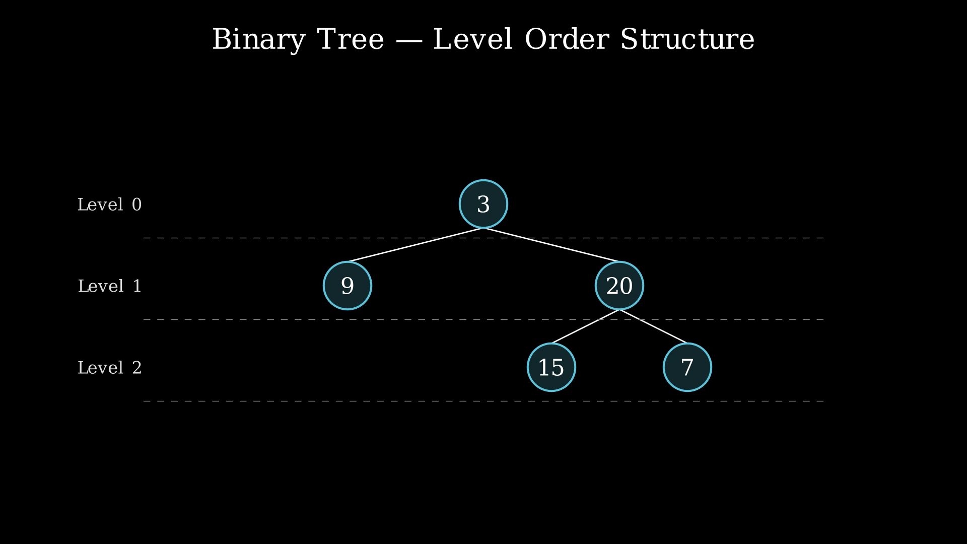
For example, in a tree with root 3, left child 9, and right child 20 (which itself has children 15 and 7), the level order traversal produces [[3], [9, 20], [15, 7]] — first the root level, then all nodes at depth 1, then all nodes at depth 2.
Examples
Example 1
Input: root = [3, 9, 20, null, null, 15, 7]
Output: [[3], [9, 20], [15, 7]]
Explanation: The tree has three levels. Level 0 contains only the root node with value 3. Level 1 contains nodes 9 (left child of 3) and 20 (right child of 3). Level 2 contains nodes 15 (left child of 20) and 7 (right child of 20). Node 9 has no children, so no nodes appear below it at level 2 on the left side.
Example 2
Input: root = [1]
Output: [[1]]
Explanation: The tree contains a single node. It sits alone at level 0. The result is a list containing one inner list with just the value 1.
Example 3
Input: root = []
Output: []
Explanation: An empty tree has no nodes at all, so the result is an empty list. This is an important edge case — always check whether the root is null before processing.
Constraints
- The number of nodes in the tree is in the range [0, 2000]
- -1000 ≤ Node.val ≤ 1000
Editorial
Brute Force
Intuition
The most natural first instinct is to use Depth-First Search (DFS) — a recursive traversal that dives deep into the tree before backtracking. While DFS naturally processes nodes in a top-to-bottom, left-to-right order within each subtree, it does not naturally group nodes by level.
To work around this, we pass the current depth as a parameter during the recursion. Whenever we visit a node, we place its value into the list corresponding to its depth. If we visit a node at depth 2, its value goes into the third inner list (index 2).
Imagine you are exploring floors of a building by taking the stairs. You might go from floor 0 to floor 2 on the left staircase, then backtrack to floor 1, then go down the right staircase to floor 2 again. At the end, you group your notes by floor number — that is exactly what this DFS approach does.
This works correctly and is actually efficient, but it is not the textbook approach for level order traversal. The natural and more intuitive way to process nodes level by level is Breadth-First Search (BFS), which we will explore next.
Step-by-Step Explanation
Let's trace through with the tree root = [3, 9, 20, null, null, 15, 7]:
Step 1: Call dfs(node=3, depth=0). Depth 0 has no list yet → create it. result = [[3]].
Step 2: Recurse left: dfs(node=9, depth=1). Depth 1 has no list yet → create it. result = [[3], [9]].
Step 3: Recurse left from 9: dfs(null, depth=2). Node is null → return immediately. No action.
Step 4: Recurse right from 9: dfs(null, depth=2). Node is null → return immediately. Back to node 9, then back to node 3.
Step 5: Recurse right from 3: dfs(node=20, depth=1). Depth 1 already exists → append 20. result = [[3], [9, 20]].
Step 6: Recurse left from 20: dfs(node=15, depth=2). Depth 2 has no list yet → create it. result = [[3], [9, 20], [15]].
Step 7: Node 15 has no children (both null). Return to node 20.
Step 8: Recurse right from 20: dfs(node=7, depth=2). Depth 2 exists → append 7. result = [[3], [9, 20], [15, 7]].
Step 9: Node 7 has no children. Return up the call stack.
Result: [[3], [9, 20], [15, 7]]
DFS with Depth Tracking — Recursive Level Grouping — Watch how DFS dives deep into the tree and uses the depth parameter to place each node's value into the correct level list, building the result as it backtracks.
Algorithm
- Create an empty result list
- Define a recursive function dfs(node, depth):
a. If node is null, return
b. If result has no list at index depth, create a new empty list
c. Append node.val to result[depth]
d. Recurse: dfs(node.left, depth + 1)
e. Recurse: dfs(node.right, depth + 1) - Call dfs(root, 0)
- Return result
Code
class Solution {
public:
    vector<vector<int>> levelOrder(TreeNode* root) {
        vector<vector<int>> result;
        dfs(root, 0, result);
        return result;
    }

    void dfs(TreeNode* node, int depth, vector<vector<int>>& result) {
        if (!node) return;

        if (depth == result.size()) {
            result.push_back({});
        }

        result[depth].push_back(node->val);
        dfs(node->left, depth + 1, result);
        dfs(node->right, depth + 1, result);
    }
};
class Solution:
def levelOrder(self, root: Optional[TreeNode]) -> list[list[int]]:
result = []
def dfs(node, depth):
if not node:
return
if depth == len(result):
result.append([])
result[depth].append(node.val)
dfs(node.left, depth + 1)
dfs(node.right, depth + 1)
dfs(root, 0)
return resultclass Solution {
public List<List<Integer>> levelOrder(TreeNode root) {
List<List<Integer>> result = new ArrayList<>();
dfs(root, 0, result);
return result;
}
private void dfs(TreeNode node, int depth, List<List<Integer>> result) {
if (node == null) return;
if (depth == result.size()) {
result.add(new ArrayList<>());
}
result.get(depth).add(node.val);
dfs(node.left, depth + 1, result);
dfs(node.right, depth + 1, result);
}
}Complexity Analysis
Time Complexity: O(n)
We visit every node in the tree exactly once. At each node, we perform O(1) work — checking the depth, appending to a list, and making two recursive calls. Since there are n nodes total, the time is O(n).
Space Complexity: O(n)
The result list stores all n node values, requiring O(n) space. Additionally, the recursion stack can go as deep as the height of the tree. In the worst case (a completely skewed tree), the height is n, giving O(n) recursion depth. In the best case (balanced tree), the height is O(log n). The overall space is O(n) dominated by the output.
Why This Approach Is Not Efficient
The DFS approach works correctly and runs in O(n) time, which is asymptotically optimal — we must visit every node at least once. However, it has a conceptual drawback and a practical one:
Conceptual drawback: Level order traversal is inherently a breadth-first concept — we want to process all nodes at one depth before moving to the next. DFS processes nodes depth-first, diving deep before going wide. We had to artificially reconstruct the level grouping using a depth parameter. The result is correct, but the approach fights against the natural structure of the problem.
Practical drawback: In a skewed tree (essentially a linked list), the recursion stack depth becomes O(n), which can cause a stack overflow for very deep trees. BFS uses a queue that is bounded by the maximum width of the tree, which is at most O(n) but typically much smaller.
The key insight: Breadth-First Search (BFS) naturally visits nodes level by level. By using a queue and processing all nodes at the current level before moving to the next, we get the level grouping for free — without needing a depth parameter or recursion.
Optimal Approach - BFS with Queue
Intuition
Breadth-First Search (BFS) is the natural algorithm for level order traversal. It uses a queue — a first-in, first-out (FIFO) data structure — to process nodes in the order they are discovered.
The idea is simple: start by putting the root into the queue. Then, repeatedly do the following: count how many nodes are currently in the queue (this is the number of nodes at the current level), process all of them one by one, and for each node processed, add its children to the queue. After processing all nodes at the current level, the queue now contains exactly the nodes at the next level.
Think of it like a school fire drill. All students on the first floor exit first (level 0). As they leave, they tell students on the second floor to start moving (their children enter the queue). Once the first floor is clear, all second-floor students exit (level 1), and so on. Each floor is fully evacuated before moving to the next.
This approach naturally groups nodes by level because we process the entire queue contents (one level) before any nodes from the next level are processed.
Step-by-Step Explanation
Let's trace through with root = [3, 9, 20, null, null, 15, 7]:
Step 1: Initialize queue with the root node [3]. Result = [].
Step 2: Level 0 — queue has 1 node. Process it:
- Dequeue node 3. Add its value to level list: [3].
- Enqueue left child 9 and right child 20.
- Level 0 complete. Append [3] to result. Result = [[3]]. Queue = [9, 20].
Step 3: Level 1 — queue has 2 nodes. Process both:
- Dequeue node 9. Add 9 to level list: [9]. Node 9 has no children — nothing to enqueue.
- Dequeue node 20. Add 20 to level list: [9, 20]. Enqueue left child 15 and right child 7.
- Level 1 complete. Append [9, 20] to result. Result = [[3], [9, 20]]. Queue = [15, 7].
Step 4: Level 2 — queue has 2 nodes. Process both:
- Dequeue node 15. Add 15 to level list: [15]. No children.
- Dequeue node 7. Add 7 to level list: [15, 7]. No children.
- Level 2 complete. Append [15, 7] to result. Result = [[3], [9, 20], [15, 7]]. Queue = [].
Step 5: Queue is empty — all levels processed.
Result: [[3], [9, 20], [15, 7]]
BFS Level Order — Queue-Based Traversal — Watch how the queue processes all nodes at one level before moving to the next, naturally grouping nodes by depth without needing a depth parameter.
Algorithm
- If root is null, return an empty list
- Initialize a queue and enqueue the root node
- While the queue is not empty:
a. Record the current queue size (level_size) — this is the number of nodes at the current level
b. Create an empty list for the current level
c. For i from 0 to level_size - 1:- Dequeue a node
- Add its value to the current level list
- If it has a left child, enqueue the left child
- If it has a right child, enqueue the right child
d. Append the current level list to the result
- Return the result
Code
class Solution {
public:
    vector<vector<int>> levelOrder(TreeNode* root) {
        vector<vector<int>> result;
        if (!root) return result;

        queue<TreeNode*> q;
        q.push(root);

        while (!q.empty()) {
            int levelSize = q.size();
            vector<int> level;

            for (int i = 0; i < levelSize; i++) {
                TreeNode* node = q.front();
                q.pop();
                level.push_back(node->val);

                if (node->left) q.push(node->left);
                if (node->right) q.push(node->right);
            }

            result.push_back(level);
        }

        return result;
    }
};
from collections import deque
class Solution:
def levelOrder(self, root: Optional[TreeNode]) -> list[list[int]]:
if not root:
return []
result = []
queue = deque([root])
while queue:
level_size = len(queue)
level = []
for _ in range(level_size):
node = queue.popleft()
level.append(node.val)
if node.left:
queue.append(node.left)
if node.right:
queue.append(node.right)
result.append(level)
return resultclass Solution {
public List<List<Integer>> levelOrder(TreeNode root) {
List<List<Integer>> result = new ArrayList<>();
if (root == null) return result;
Queue<TreeNode> queue = new LinkedList<>();
queue.offer(root);
while (!queue.isEmpty()) {
int levelSize = queue.size();
List<Integer> level = new ArrayList<>();
for (int i = 0; i < levelSize; i++) {
TreeNode node = queue.poll();
level.add(node.val);
if (node.left != null) queue.offer(node.left);
if (node.right != null) queue.offer(node.right);
}
result.add(level);
}
return result;
}
}Complexity Analysis
Time Complexity: O(n)
Every node is enqueued and dequeued exactly once. Each enqueue and dequeue operation is O(1). We also do O(1) work per node (adding value to the level list, checking children). Total: n × O(1) = O(n).
Space Complexity: O(n)
The result list stores all n values, requiring O(n). The queue at any point holds at most the nodes of one level. In the worst case (a complete binary tree), the widest level has approximately n/2 nodes, so the queue uses O(n) space. In a skewed tree, the queue holds at most 1 node at a time, but the result still requires O(n). Overall: O(n).
Compared to DFS, BFS avoids the risk of O(n) recursion depth in skewed trees. The queue-based approach is iterative, so it uses heap memory (for the queue) rather than stack memory (for recursion), which is more robust for very deep trees.