Unique Paths
Description
A robot is placed on an m × n grid at the top-left corner (cell (0, 0)). The robot wants to reach the bottom-right corner (cell (m - 1, n - 1)). At any point in time, the robot can only move down or right — it cannot move up, left, or diagonally.
Given the two integers m (rows) and n (columns), return the total number of unique paths the robot can take to travel from the top-left corner to the bottom-right corner.
The answer is guaranteed to be less than or equal to 2 × 10⁹.
Examples
Example 1
Input: m = 3, n = 7
Output: 28
Explanation: The robot starts at cell (0, 0) on a 3×7 grid and must reach cell (2, 6). It must make exactly 2 downward moves and 6 rightward moves (in some order). The total number of distinct orderings of these moves is 28.
Example 2
Input: m = 3, n = 2
Output: 3
Explanation: From the top-left corner, there are exactly 3 ways to reach the bottom-right corner:
- Right → Down → Down
- Down → Down → Right
- Down → Right → Down
Example 3
Input: m = 3, n = 3
Output: 6
Explanation: On a 3×3 grid, the robot must make 2 down moves and 2 right moves. There are 6 distinct ways to interleave these moves to reach cell (2, 2) from cell (0, 0).
Constraints
- 1 ≤ m, n ≤ 100
Editorial
Brute Force
Intuition
The most natural way to think about this problem is to explore every possible route the robot can take. At each cell, the robot has at most two choices: move right or move down. If we try every combination of these two choices, we will eventually enumerate all paths from the top-left to the bottom-right.
Imagine you are standing at an intersection in a city grid. At every intersection, you can only go east or south. To count all the routes from the northwest corner to the southeast corner, you could physically walk every possible route — that is what recursion does for us. Each recursive call represents one step in one direction, and when we reach the destination, we count that as one valid path.
Step-by-Step Explanation
Let's trace through with m = 3, n = 3 (a 3×3 grid). We call countPaths(0, 0) and explore all branches:
Step 1: Start at cell (0, 0). We can go right to (0, 1) or down to (1, 0).
Step 2: Explore the right branch — call countPaths(0, 1). From (0, 1), we can go right to (0, 2) or down to (1, 1).
Step 3: Explore countPaths(0, 2). From (0, 2), we can only go down since column 2 is the last column. Go to (1, 2).
Step 4: From (1, 2), go down to (2, 2). This is the destination! Count this as 1 valid path. Return 1 up the call chain.
Step 5: Back at (0, 1), now explore the down branch — countPaths(1, 1). From (1, 1), we can go right to (1, 2) or down to (2, 1).
Step 6: countPaths(1, 2): go down to (2, 2) — destination reached. Return 1.
Step 7: countPaths(2, 1): go right to (2, 2) — destination reached. Return 1.
Step 8: countPaths(1, 1) returns 1 + 1 = 2. So countPaths(0, 1) returns 1 + 2 = 3.
Step 9: Back at (0, 0), explore the down branch — countPaths(1, 0). Similarly, this branch explores (1, 1), (2, 0), and their sub-branches.
Step 10: countPaths(1, 0) eventually returns 3. So countPaths(0, 0) returns 3 + 3 = 6.
Result: There are 6 unique paths in a 3×3 grid.
Recursive Exploration of All Paths (3×3 Grid) — Watch how the recursion branches at every cell, exploring all right/down combinations until reaching the destination (2,2). Many subproblems like (1,1) are computed repeatedly.
Algorithm
- Define a recursive function
countPaths(i, j)that returns the number of unique paths from cell (i, j) to cell (m-1, n-1) - Base case: If
i == m - 1andj == n - 1, we have reached the destination — return 1 - Out of bounds: If
i >= morj >= n, we have gone outside the grid — return 0 - Recursive case: Return
countPaths(i + 1, j) + countPaths(i, j + 1)— the sum of paths from moving down and moving right - Call
countPaths(0, 0)to get the answer
Code
class Solution {
public:
    int countPaths(int i, int j, int m, int n) {
        // Reached destination
        if (i == m - 1 && j == n - 1)
            return 1;

        // Out of bounds
        if (i >= m || j >= n)
            return 0;

        // Move down + move right
        return countPaths(i + 1, j, m, n) + countPaths(i, j + 1, m, n);
    }

    int uniquePaths(int m, int n) {
        return countPaths(0, 0, m, n);
    }
};
class Solution:
def uniquePaths(self, m: int, n: int) -> int:
def count_paths(i: int, j: int) -> int:
# Reached destination
if i == m - 1 and j == n - 1:
return 1
# Out of bounds
if i >= m or j >= n:
return 0
# Move down + move right
return count_paths(i + 1, j) + count_paths(i, j + 1)
return count_paths(0, 0)class Solution {
private int countPaths(int i, int j, int m, int n) {
// Reached destination
if (i == m - 1 && j == n - 1)
return 1;
// Out of bounds
if (i >= m || j >= n)
return 0;
// Move down + move right
return countPaths(i + 1, j, m, n) + countPaths(i, j + 1, m, n);
}
public int uniquePaths(int m, int n) {
return countPaths(0, 0, m, n);
}
}Complexity Analysis
Time Complexity: O(2^(m+n))
At each cell, the function branches into two recursive calls (down and right). The maximum depth of recursion is (m - 1) + (n - 1) = m + n - 2, and the tree can have up to 2^(m+n-2) nodes. This exponential growth makes it impractical for large grids.
Space Complexity: O(m + n)
The recursion stack can go at most m + n - 2 levels deep (one step per row or column traversed). Each stack frame uses constant space, so the total space is proportional to the depth of the recursion tree.
Why This Approach Is Not Efficient
The brute force recursion has exponential time complexity O(2^(m+n)) because it recomputes the same subproblems over and over. For instance, the number of paths from cell (1, 1) to the destination is computed multiple times — once when reached from (0, 1) going down, and again when reached from (1, 0) going right.
With constraints allowing m and n up to 100, the recursion tree could have up to 2^198 nodes — a number so astronomically large that it would take longer than the age of the universe to compute. Even for modest grids like 10×10, the brute force makes thousands of redundant calls.
The key observation is that the result for any cell (i, j) depends only on i and j — not on how we got there. There are only m × n unique cells, so at most m × n unique subproblems exist. By storing already-computed results, we can eliminate all redundancy.
Better Approach - Dynamic Programming (Tabulation)
Intuition
Instead of recursing from the start and recomputing overlapping subproblems, we can build the answer from the bottom up using a 2D table.
Think of it this way: how many ways can you reach each cell in the grid? For any cell in the first row, there is exactly one way — go right, right, right. For any cell in the first column, there is also exactly one way — go down, down, down. For every other cell (i, j), you could have arrived from the cell above (i-1, j) or from the cell to the left (i, j-1). So the number of ways to reach (i, j) is the sum of ways to reach those two neighbors.
This is like filling in a multiplication-table-style grid: start by writing 1 in the entire first row and first column, then fill each remaining cell as the sum of the cell above it and the cell to its left.
Step-by-Step Explanation
Let's trace through with m = 3, n = 3:
Step 1: Create a 3×3 DP table. Initialize all cells in the first row to 1 (only one way to reach any cell in the top row — keep going right).
Step 2: Initialize all cells in the first column to 1 (only one way to reach any cell in the leftmost column — keep going down).
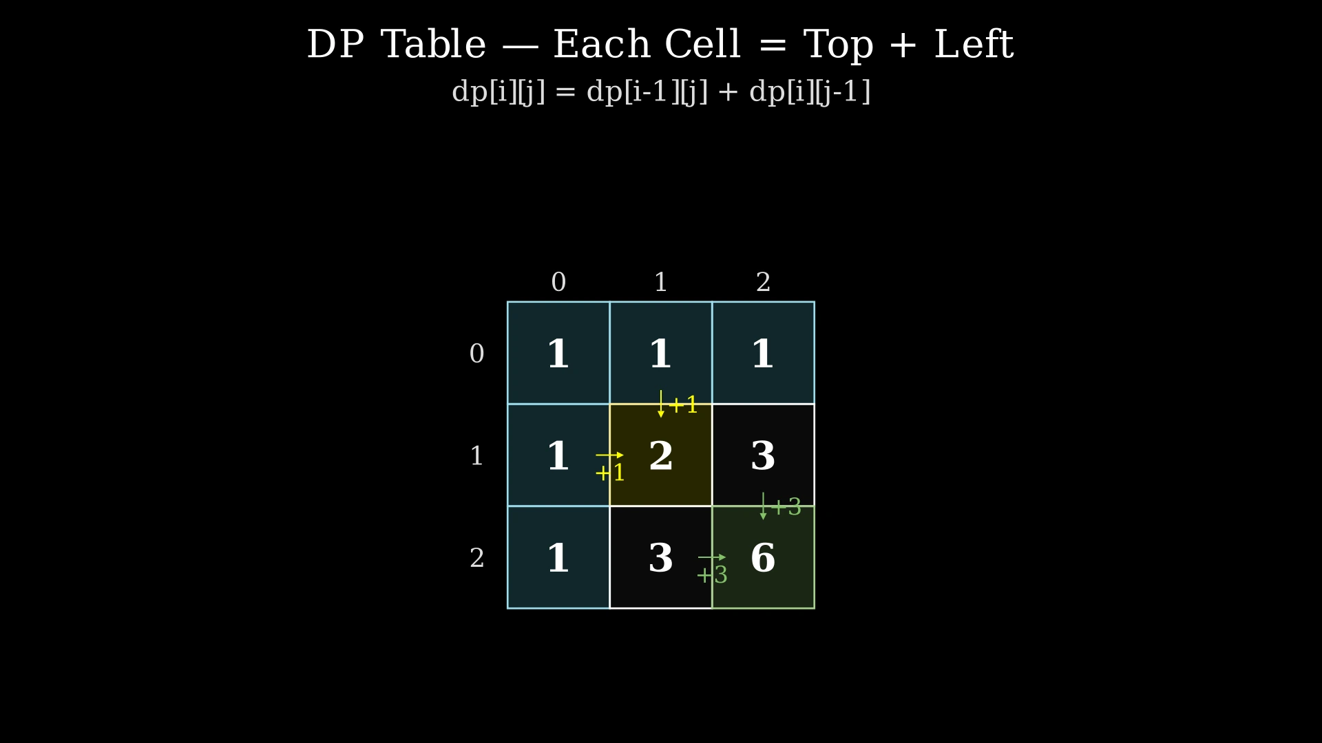
Step 3: Fill cell (1, 1): dp[1][1] = dp[0][1] + dp[1][0] = 1 + 1 = 2. There are 2 ways to reach (1,1).
Step 4: Fill cell (1, 2): dp[1][2] = dp[0][2] + dp[1][1] = 1 + 2 = 3. There are 3 ways to reach (1,2).
Step 5: Fill cell (2, 1): dp[2][1] = dp[1][1] + dp[2][0] = 2 + 1 = 3. There are 3 ways to reach (2,1).
Step 6: Fill cell (2, 2): dp[2][2] = dp[1][2] + dp[2][1] = 3 + 3 = 6. There are 6 ways to reach the destination.
Result: dp[2][2] = 6 unique paths.
Bottom-Up DP Table Construction (3×3 Grid) — Watch the DP table fill cell by cell. Each cell's value is the sum of the cell directly above it and the cell to its left, representing the total number of paths to reach that cell.
Algorithm
- Create a 2D array
dpof size m × n - Initialize the first row:
dp[0][j] = 1for all j (only one path — all right moves) - Initialize the first column:
dp[i][0] = 1for all i (only one path — all down moves) - For each remaining cell (i, j) where i ≥ 1 and j ≥ 1:
dp[i][j] = dp[i-1][j] + dp[i][j-1]
- Return
dp[m-1][n-1]
Code
class Solution {
public:
    int uniquePaths(int m, int n) {
        vector<vector<int>> dp(m, vector<int>(n, 1));

        for (int i = 1; i < m; i++) {
            for (int j = 1; j < n; j++) {
                dp[i][j] = dp[i - 1][j] + dp[i][j - 1];
            }
        }

        return dp[m - 1][n - 1];
    }
};
class Solution:
def uniquePaths(self, m: int, n: int) -> int:
dp = [[1] * n for _ in range(m)]
for i in range(1, m):
for j in range(1, n):
dp[i][j] = dp[i - 1][j] + dp[i][j - 1]
return dp[m - 1][n - 1]class Solution {
public int uniquePaths(int m, int n) {
int[][] dp = new int[m][n];
// Initialize first row and first column to 1
for (int i = 0; i < m; i++) dp[i][0] = 1;
for (int j = 0; j < n; j++) dp[0][j] = 1;
for (int i = 1; i < m; i++) {
for (int j = 1; j < n; j++) {
dp[i][j] = dp[i - 1][j] + dp[i][j - 1];
}
}
return dp[m - 1][n - 1];
}
}Complexity Analysis
Time Complexity: O(m × n)
We iterate through every cell of the m × n grid exactly once. The computation at each cell (one addition) takes O(1) time, so the total work is m × n operations.
Space Complexity: O(m × n)
We store the entire 2D DP table of size m × n. For the maximum constraints (m = n = 100), this means storing 10,000 integers — very manageable.
Why This Approach Is Not Efficient
The 2D DP tabulation approach runs in O(m × n) time, which is efficient enough for the given constraints. However, it uses O(m × n) space for the full DP table.
Looking closely at the recurrence dp[i][j] = dp[i-1][j] + dp[i][j-1], we observe that to fill row i, we only need values from row i - 1 (the row directly above) and the current row (values to the left). We never look back at row i - 2 or earlier. This means we are storing many rows of data that are no longer needed.
We can reduce space from O(m × n) down to O(n) by using a single 1D array and updating it row by row. But even this still requires O(m × n) time.
For an even more efficient solution, we can use a mathematical formula that runs in O(min(m, n)) time with O(1) space.
Optimal Approach - Combinatorics
Intuition
Here is a powerful mathematical insight: every path from (0, 0) to (m-1, n-1) consists of exactly the same number of moves — you must make (m - 1) downward moves and (n - 1) rightward moves. The total number of moves is (m - 1) + (n - 1) = m + n - 2.
Each unique path is simply a different ordering of these fixed moves. The question becomes: in how many ways can we arrange (m - 1) D's and (n - 1) R's in a sequence of length (m + n - 2)?
This is a classic combinatorics problem. The answer is the binomial coefficient:
C(m + n - 2, m - 1) = (m + n - 2)! / ((m - 1)! × (n - 1)!)
Think of it like choosing seats on a bus: you have m + n - 2 total seats (moves), and you need to pick which m - 1 of them will be "down" moves. The remaining seats automatically become "right" moves. The number of ways to choose is the combination formula.
For the 3×3 example: total moves = 4, down moves = 2. C(4, 2) = 4! / (2! × 2!) = 24 / 4 = 6. This matches our DP result!
Step-by-Step Explanation
Let's trace through with m = 3, n = 7:
Step 1: Compute the total number of moves: total = m + n - 2 = 3 + 7 - 2 = 8. Every path has exactly 8 steps.
Step 2: Compute the number of down moves: downs = m - 1 = 2. (We could equivalently choose rights = n - 1 = 6; we pick the smaller for efficiency.)
Step 3: We need r = min(m - 1, n - 1) = min(2, 6) = 2. We compute C(8, 2).
Step 4: Begin iterative computation. Start with path = 1.
- i = 1: path = path × (total - r + i) / i = 1 × (8 - 2 + 1) / 1 = 1 × 7 / 1 = 7
Step 5: Continue:
- i = 2: path = path × (8 - 2 + 2) / 2 = 7 × 8 / 2 = 56 / 2 = 28
Step 6: r iterations complete. The answer is path = 28.
Result: C(8, 2) = 28 unique paths.
Computing C(8, 2) Iteratively — Unique Paths for 3×7 Grid — Watch the combinatorial formula C(m+n-2, min(m-1,n-1)) compute the answer iteratively, multiplying and dividing one factor at a time to avoid integer overflow.
Algorithm
- Compute
total = m + n - 2(total number of moves in any path) - Compute
r = min(m - 1, n - 1)(choose the smaller value for fewer iterations) - Initialize
path = 1 - For
ifrom 1 tor:- Multiply:
path = path × (total - r + i) / i - This incrementally computes C(total, r) without computing full factorials
- Multiply:
- Return
path
Code
class Solution {
public:
    int uniquePaths(int m, int n) {
        int total = m + n - 2;
        int r = min(m - 1, n - 1);

        long long path = 1;
        for (int i = 1; i <= r; i++) {
            path = path * (total - r + i) / i;
        }

        return (int)path;
    }
};
class Solution:
def uniquePaths(self, m: int, n: int) -> int:
total = m + n - 2
r = min(m - 1, n - 1)
path = 1
for i in range(1, r + 1):
path = path * (total - r + i) // i
return pathclass Solution {
public int uniquePaths(int m, int n) {
int total = m + n - 2;
int r = Math.min(m - 1, n - 1);
long path = 1;
for (int i = 1; i <= r; i++) {
path = path * (total - r + i) / i;
}
return (int) path;
}
}Complexity Analysis
Time Complexity: O(min(m, n))
The loop runs r = min(m - 1, n - 1) times. Each iteration involves one multiplication and one division — both O(1) operations. For the maximum constraints (m = n = 100), this is just 99 iterations.
Space Complexity: O(1)
We use only a few variables (total, r, path, i). No arrays or matrices are needed. This is a dramatic improvement over the O(m × n) space of the DP approach.