Permutations
Description
Given an array of distinct integers, return all possible permutations of those integers. A permutation is a rearrangement of all elements where the order matters — different orderings count as different permutations.
For example, the array [1, 2] has two permutations: [1, 2] and [2, 1]. You need to find every such rearrangement for the given input.
You can return the permutations in any order.
Examples
Example 1
Input: nums = [1, 2, 3]
Output: [[1,2,3], [1,3,2], [2,1,3], [2,3,1], [3,1,2], [3,2,1]]
Explanation: There are 3! = 6 ways to arrange three distinct elements. Each permutation uses all three numbers exactly once, in a different order.
Example 2
Input: nums = [0, 1]
Output: [[0,1], [1,0]]
Explanation: With two elements, there are only 2! = 2 possible orderings: the original and the reversed.
Example 3
Input: nums = [1]
Output: [[1]]
Explanation: A single element has only one permutation — itself.
Constraints
- 1 ≤ nums.length ≤ 6
- -10 ≤ nums[i] ≤ 10
- All the integers of nums are unique
Editorial
Brute Force - Iterative Insertion
Intuition
Imagine you have numbered tiles and want to find every possible arrangement. A natural approach is to build permutations one element at a time.
Start with just the first tile. There is only one way to arrange one tile. Now pick up the second tile and try inserting it at every possible position in your existing arrangement — before the first tile, or after it. Each insertion creates a new arrangement. For each of those arrangements, pick up the third tile and insert it at every possible position.
This is the iterative insertion approach: at each round, we take the next element and create new permutations by slotting it into every possible position within every existing permutation. After processing all elements, every permutation has been constructed.
Step-by-Step Explanation
Let's trace through with nums = [1, 2, 3]:
Step 1: Start with the first element. We have exactly one permutation: [[1]].
Step 2: Take element 2. Insert it at position 0 (before 1) in [1] → we get [2, 1].
Step 3: Insert element 2 at position 1 (after 1) in [1] → we get [1, 2]. Round complete. Current permutations: [[2, 1], [1, 2]].
Step 4: Take element 3. Insert it at position 0 of [2, 1] → [3, 2, 1].
Step 5: Insert 3 at position 1 of [2, 1] → [2, 3, 1]. The 3 slides between 2 and 1.
Step 6: Insert 3 at position 2 of [2, 1] → [2, 1, 3]. All positions for source [2, 1] exhausted.
Step 7: Switch to next source. Insert 3 at position 0 of [1, 2] → [3, 1, 2].
Step 8: Insert 3 at position 1 of [1, 2] → [1, 3, 2].
Step 9: Insert 3 at position 2 of [1, 2] → [1, 2, 3]. All insertions done. Final result: 6 permutations, which equals 3! as expected.
Iterative Insertion — Building Permutations Round by Round — Watch how permutations are built by inserting each new element at every possible position. The main array shows the source permutation, and the secondary array shows the newly created permutation after each insertion.
Algorithm
- Initialize the result list with a single permutation containing only the first element: [[nums[0]]]
- For each remaining element nums[i] (i from 1 to n-1):
- Create an empty list for new permutations
- For each existing permutation in the result:
- For each position j from 0 to the length of that permutation:
- Create a copy of the permutation
- Insert nums[i] at position j in the copy
- Add the new permutation to the new list
- For each position j from 0 to the length of that permutation:
- Replace result with the new list
- Return result
Code
#include <vector>
using namespace std;

class Solution {
public:
    vector<vector<int>> permute(vector<int>& nums) {
        vector<vector<int>> result = {{nums[0]}};

        for (int i = 1; i < (int)nums.size(); i++) {
            vector<vector<int>> newPerms;
            for (auto& perm : result) {
                for (int j = 0; j <= (int)perm.size(); j++) {
                    vector<int> copy = perm;
                    copy.insert(copy.begin() + j, nums[i]);
                    newPerms.push_back(copy);
                }
            }
            result = newPerms;
        }

        return result;
    }
};
class Solution:
def permute(self, nums: list[int]) -> list[list[int]]:
result = [[nums[0]]]
for i in range(1, len(nums)):
new_perms = []
for perm in result:
for j in range(len(perm) + 1):
new_perm = perm[:j] + [nums[i]] + perm[j:]
new_perms.append(new_perm)
result = new_perms
return resultimport java.util.*;
class Solution {
public List<List<Integer>> permute(int[] nums) {
List<List<Integer>> result = new ArrayList<>();
List<Integer> first = new ArrayList<>();
first.add(nums[0]);
result.add(first);
for (int i = 1; i < nums.length; i++) {
List<List<Integer>> newPerms = new ArrayList<>();
for (List<Integer> perm : result) {
for (int j = 0; j <= perm.size(); j++) {
List<Integer> copy = new ArrayList<>(perm);
copy.add(j, nums[i]);
newPerms.add(copy);
}
}
result = newPerms;
}
return result;
}
}Complexity Analysis
Time Complexity: O(n × n!)
At round k, we have k! permutations of length k. For each, we insert the next element at (k+1) positions, producing (k+1)! new permutations. Each insertion involves copying a list of length k, costing O(k). Summing across all rounds gives O(n × n!).
Space Complexity: O(n × n!)
At any point during construction, we store all current permutations. At the final round we hold n! permutations each of length n, giving O(n × n!) space. During each round we temporarily hold both the old and new permutation lists, roughly doubling the memory before the old list is discarded.
Why This Approach Is Not Efficient
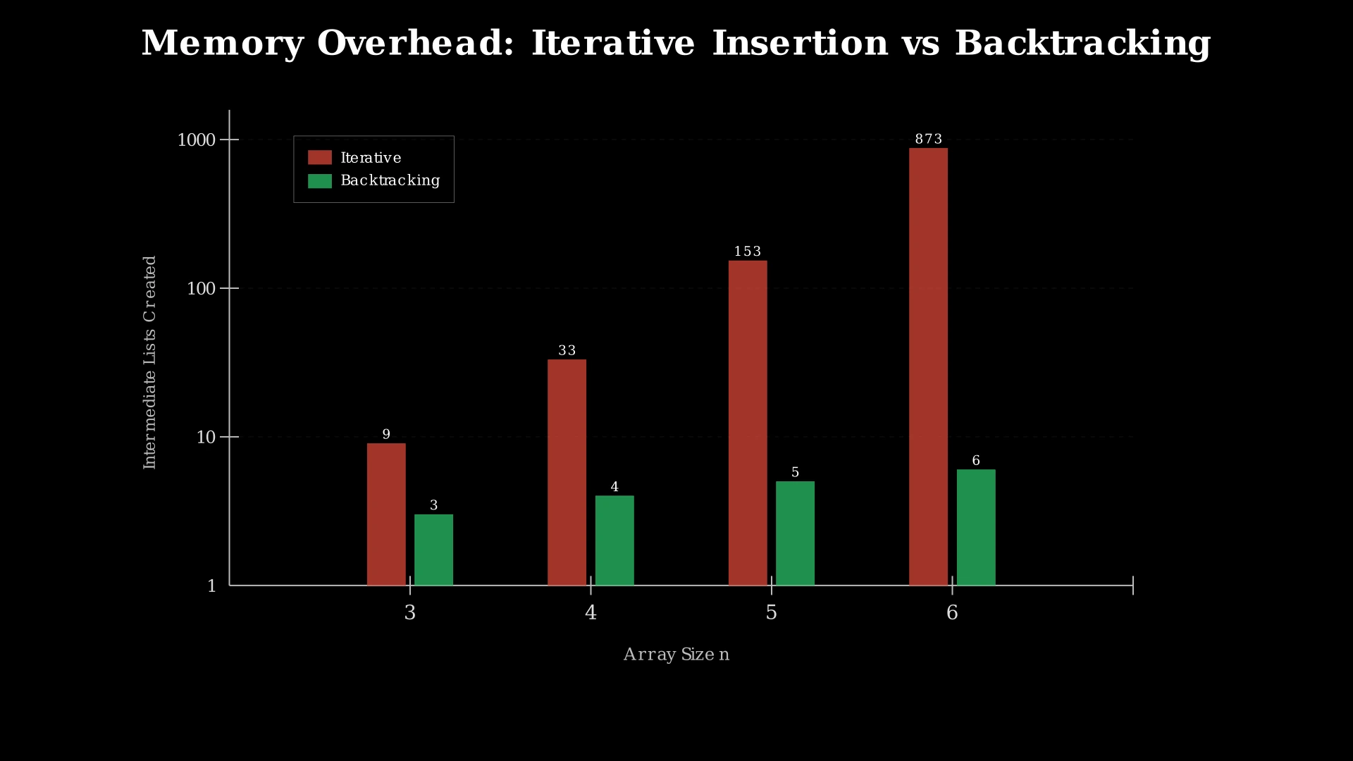
While the iterative insertion approach correctly generates all permutations, it is wasteful with memory. At each round, it stores all intermediate permutations and creates brand-new list copies for every single insertion.
For an array of size n = 6, the final round alone produces 720 permutations. But during construction, we also hold the previous 120 permutations temporarily, and every insertion requires copying an entire list. The total number of intermediate lists created across all rounds is 1! + 2! + 3! + 4! + 5! + 6! = 873.
The core issue is that this approach builds permutations "from the outside in" — it never reuses memory. Every new permutation is a fresh copy.
A smarter strategy is to build permutations "in-place" by swapping elements within the original array. Instead of creating hundreds of separate lists during construction, we manipulate one array and only make a copy when we find a complete permutation. This is exactly what backtracking with swaps achieves — same time complexity but dramatically less memory overhead.
Optimal Approach - Backtracking with Swap
Intuition
Think of building a permutation as making a sequence of decisions. At position 0, you choose which element goes there. At position 1, you choose from the remaining elements. At position 2, from whatever is left, and so on.
This naturally forms a decision tree. Each path from root to leaf represents one complete permutation. The backtracking approach explores this tree depth-first: go as deep as possible, record the result, then back up and try a different choice.
The clever trick is using swaps instead of a separate "used" tracking array. To try element nums[i] at position start, we simply swap nums[start] with nums[i]. Now nums[start] holds our choice, and all unchosen elements conveniently sit in positions start+1 through n-1. After exploring all permutations with this choice, we swap back (backtrack) to restore the original order and try the next option.
This in-place approach means we never allocate extra arrays during exploration — we only copy the array when a full permutation is completed.
![Decision tree diagram showing how backtracking generates all six permutations of [1, 2, 3]](https://pub-a1b3030acfb94e84ba8a89fb182c53bc.r2.dev/public/46/backtrack_tree_v1.webp)
Step-by-Step Explanation
Let's trace the backtracking approach with nums = [1, 2, 3]:
Step 1: Start at depth 0 with array [1, 2, 3]. We can place element 1, 2, or 3 at position 0 by swapping.
Step 2: Try keeping 1 at position 0 — swap(0,0) is an identity swap. Array stays [1, 2, 3]. Fix position 0 and recurse to depth 1.
Step 3: At depth 1, try keeping 2 at position 1 — swap(1,1). Array: [1, 2, 3]. Recurse to depth 2. Depth equals n = 3, so all positions are filled. Record permutation #1: [1, 2, 3].
Step 4: Backtrack to depth 1. Try next option: swap(1,2). Array becomes [1, 3, 2]. Recurse to depth 2. All filled — record permutation #2: [1, 3, 2]. Both arrangements starting with 1 are done.
Step 5: Backtrack to depth 0. Undo swap(1,2) to restore [1, 2, 3]. Now try element 2 at position 0: swap(0,1) gives [2, 1, 3].
Step 6: Explore depth 1 of [2, 1, 3]: swap(1,1) keeps 1 → depth 2 → permutation #3: [2, 1, 3].
Step 7: Backtrack at depth 1. Swap(1,2) gives [2, 3, 1] → permutation #4: [2, 3, 1]. All arrangements starting with 2 done.
Step 8: Backtrack to depth 0. Restore [1, 2, 3]. Try element 3 at position 0: swap(0,2) gives [3, 2, 1]. Explore depth 1: find [3, 2, 1] and [3, 1, 2]. All 3! = 6 permutations found.
Backtracking with Swap — In-Place Permutation Generation — Watch how backtracking generates all permutations by swapping elements in place. At each depth, we try placing each remaining element at the current position by swapping, recurse deeper, then swap back to restore the array before trying the next option.
Algorithm
- Create an empty result list
- Call backtrack(nums, start = 0, result):
a. Base case: If start equals n, all positions are filled. Append a copy of nums to result and return.
b. Recursive case: For each index i from start to n - 1:- Swap nums[start] with nums[i] (place element i at position start)
- Recursively call backtrack(nums, start + 1, result)
- Swap nums[start] with nums[i] again (undo the swap to restore state)
- Return result
Code
#include <vector>
using namespace std;

class Solution {
public:
    vector<vector<int>> permute(vector<int>& nums) {
        vector<vector<int>> result;
        backtrack(nums, 0, result);
        return result;
    }

private:
    void backtrack(vector<int>& nums, int start,
                   vector<vector<int>>& result) {
        if (start == (int)nums.size()) {
            result.push_back(nums);
            return;
        }
        for (int i = start; i < (int)nums.size(); i++) {
            swap(nums[start], nums[i]);
            backtrack(nums, start + 1, result);
            swap(nums[start], nums[i]);
        }
    }
};
class Solution:
def permute(self, nums: list[int]) -> list[list[int]]:
result = []
def backtrack(start: int) -> None:
if start == len(nums):
result.append(nums[:])
return
for i in range(start, len(nums)):
nums[start], nums[i] = nums[i], nums[start]
backtrack(start + 1)
nums[start], nums[i] = nums[i], nums[start]
backtrack(0)
return resultimport java.util.*;
class Solution {
public List<List<Integer>> permute(int[] nums) {
List<List<Integer>> result = new ArrayList<>();
backtrack(nums, 0, result);
return result;
}
private void backtrack(int[] nums, int start,
List<List<Integer>> result) {
if (start == nums.length) {
List<Integer> perm = new ArrayList<>();
for (int num : nums) {
perm.add(num);
}
result.add(perm);
return;
}
for (int i = start; i < nums.length; i++) {
int temp = nums[start];
nums[start] = nums[i];
nums[i] = temp;
backtrack(nums, start + 1, result);
temp = nums[start];
nums[start] = nums[i];
nums[i] = temp;
}
}
}Complexity Analysis
Time Complexity: O(n × n!)
The recursion tree has n! leaf nodes, one per permutation. At each leaf, we copy the array in O(n) time to store the result. The total number of internal nodes is bounded by O(n!) as well (each performs an O(1) swap). Therefore the overall time is O(n × n!).
Space Complexity: O(n)
The recursion stack goes at most n levels deep, using O(n) space. We modify the input array in place, so no auxiliary arrays are needed beyond the recursion stack. The output itself takes O(n × n!) space, but this is not counted as auxiliary space since it is the required output.