Vector Databases

The search lesson ended on a cliffhanger. A customer types "cozy winter soup" into the marketplace. The dish that should win is "Hearty Pho — slow-simmered broth for cold nights." Count the shared words between query and dish: zero. The inverted index — the machine we just built a whole lesson around — shrugs. Its entire worldview is terms, and these two phrases share none.

Yet any human sees they're the same idea. The information isn't in the words; it's in the meaning — and meaning is exactly what the last family on our map stores.

The trick was defined in one breath back in the landscape lesson, and now it takes center stage: an embedding is a list of numbers a model assigns to a thing — a dish description, an image, a review — such that similar things land near each other. Meaning becomes coordinates. And once meaning is coordinates, "find me things like this" becomes geometry: nearest neighbors to a point. Similarity as a query.

In this lesson: the geometric reframe, an uncomfortable first on this map (a family whose native question has no exact shortcut), the negotiation that defines every engine in the category — and 2026's honest verdict about whether this is a family at all.

Scope, drawn firmly: this course treats vector databases as a database type. How embeddings are made, which model to choose, RAG pipelines, AI application design — all deliberately out of scope (that's a different course). Here: what the store does, what it costs, and when it earns a place in your architecture.

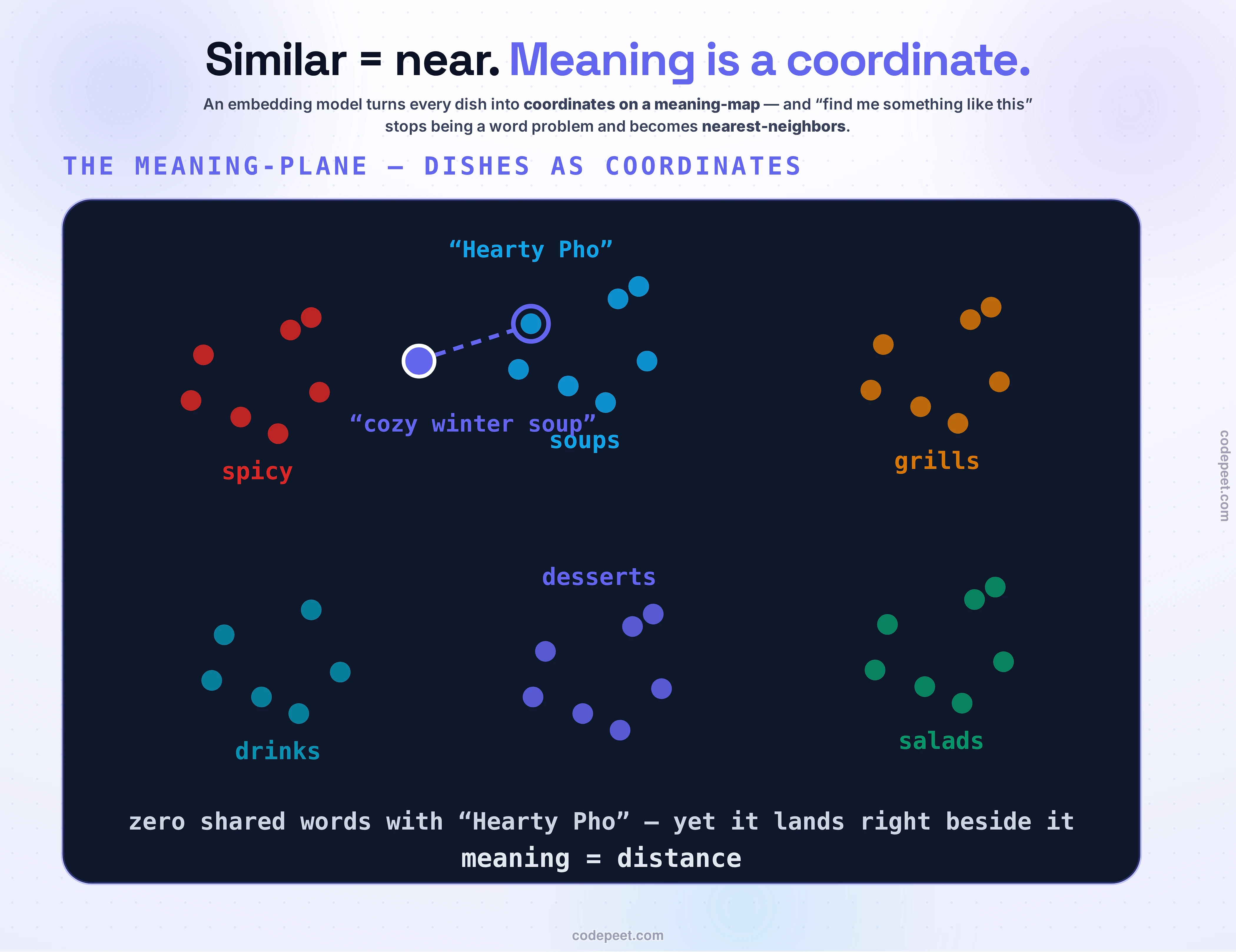
Picture the marketplace's dishes as points on a map — not a map of the city, a map of meaning. The spicy dishes cluster in one corner; soups pool together; desserts keep to themselves. "Spicy Ramen" and "Sichuan Noodles" sit almost on top of each other; "Mango Sticky Rice" lives a continent away. (The widget below renders exactly this — in 2 dimensions so you can see it; real embeddings use hundreds to a few thousand.)

Every query becomes a point too: embed "cozy winter soup" with the same model that embedded the dishes, and it lands in the soup neighborhood — right next to Hearty Pho, zero shared words and all. If that same-pipeline-on-both-sides move feels familiar, it should: it's the analyzer rule from the search lesson, reborn — matching happens in a shared representation space, never between raw inputs.

Two design choices live inside "near," and both are yours. First, the distance metric — euclidean (straight-line), cosine (angle — cares about direction of meaning, not magnitude), dot product — and swapping metrics genuinely reorders results (you'll flip between them below). Second, and this deserves emphasis precisely because it's out of scope: the database never understands anything. The embedding model decided that pho and winter-coziness are neighbors; the database just does geometry on the points it's handed. Great embeddings in, great similarity out — and confidently arranged nonsense otherwise.

Now the systems question: how do you find the nearest neighbors fast? Every previous family had a trick that made its native question exact AND cheap: hash to a shard, walk a sorted run, follow a pointer, look up a posting list. Work proportional to the question — we've hit that asymmetry three times.

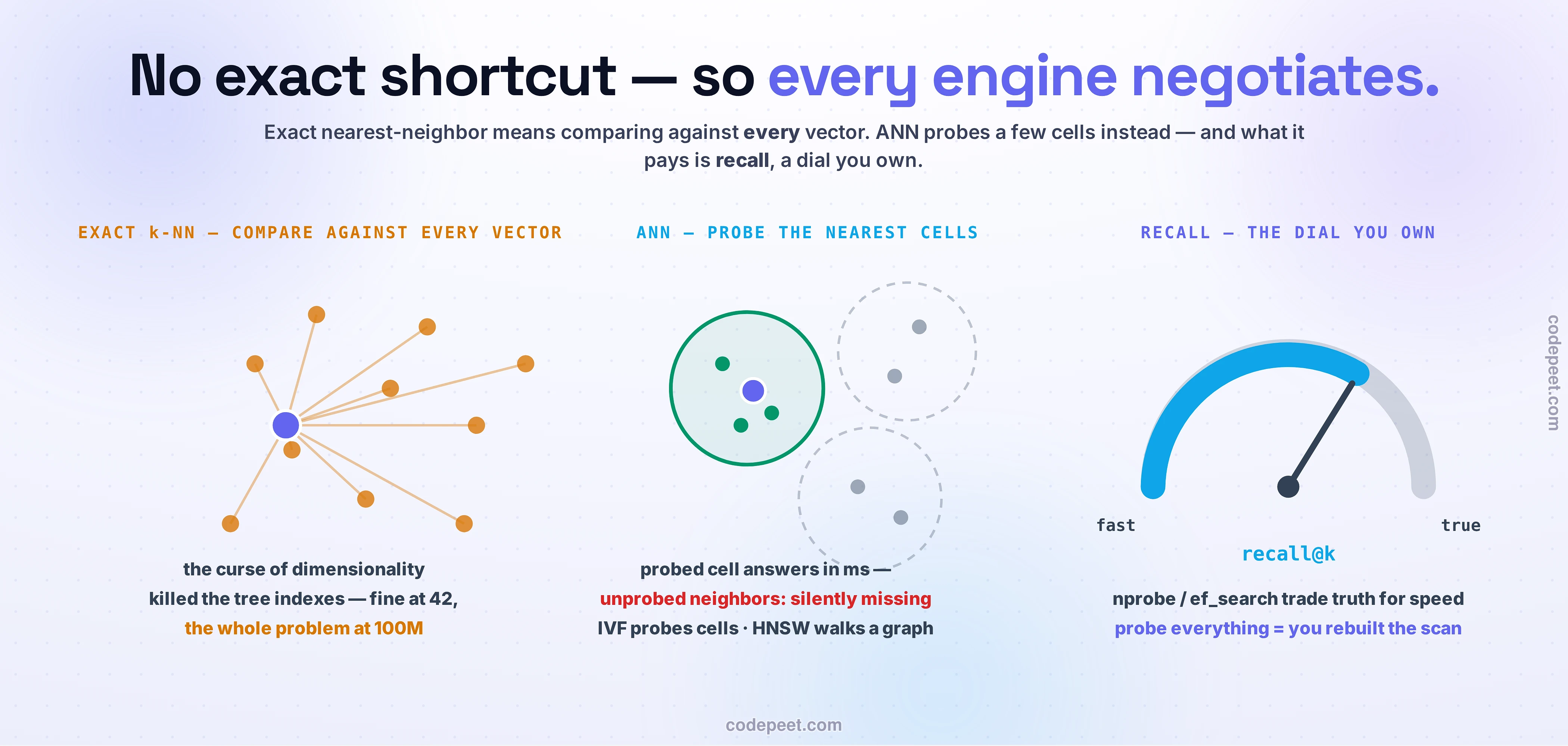
Here, for the first time, the trick doesn't exist. There is no sort order for 768-dimensional proximity — a B-tree sorts one dimension. The spatial trees that save 2-D maps (you'll meet them in Quadtrees and R-Trees) collapse in high dimensions — the curse of dimensionality: past roughly 10 dimensions their partitions stop discriminating, and at 100+ every leaf of a KD-tree sits nearly equidistant from any query. Exact nearest-neighbor means one thing: compute the distance to every single vector. A full scan, every query. Fine at 42 dishes; the entire problem at 100 million.

So this family did something no other family on the map admits to doing: it negotiated with correctness. Approximate Nearest Neighbor (ANN) indexes answer fast by accepting that the results might miss some true neighbors — and the miss rate has a name, recall@k: what fraction of the true top-k did the index actually return. Two index shapes dominate:

IVF — cluster the corpus into cells (k-means), and at query time probe only the nprobe nearest cells. Simple, memory-light — and its failure mode is built into the geometry: a query near a cell boundary has true neighbors in the next cell over, and if that cell isn't probed, they're simply absent. No error. No warning. Just quietly not the truth.

HNSW — the in-memory champion in most production engines — is a multi-layer navigable small world graph: sparse upper layers for continent-hopping, dense lower layers for street-level refinement. Read that again: the flagship vector index is a graph — greedy traversal, hub nodes, the works. The graph family from four lessons ago, moonlighting as an index. The families keep composing.

Either way, the deep takeaway is the same, and it's the one this lesson exists to install: recall is a dial, not a given. nprobe, ef_search — knobs that trade truth for speed, set by you, invisible to your users until "similar dishes" quietly stops being similar.

Below: 42 dishes on a real meaning-plane, six IVF cells, and every number computed live — real distances, real cell assignment, and recall measured against the exact answer.

The arc: with the "between spicy & soup" preset, run EXACT (all 42 distances — the guarantee and its price), then switch to ANN at nprobe=1 and meet the red rings: true neighbors, silently missing, sitting in the unprobed cell. Crank the dial and buy truth back — noticing that at nprobe=6 you've rebuilt the brute-force scan (the dial has two ends). Then flip 🌱 vegan filtering between pre and post and count what survives. Finally: click literally anywhere — it's your plane.

Three pieces of fine print separate demo-ware from production here — you just drove the first.

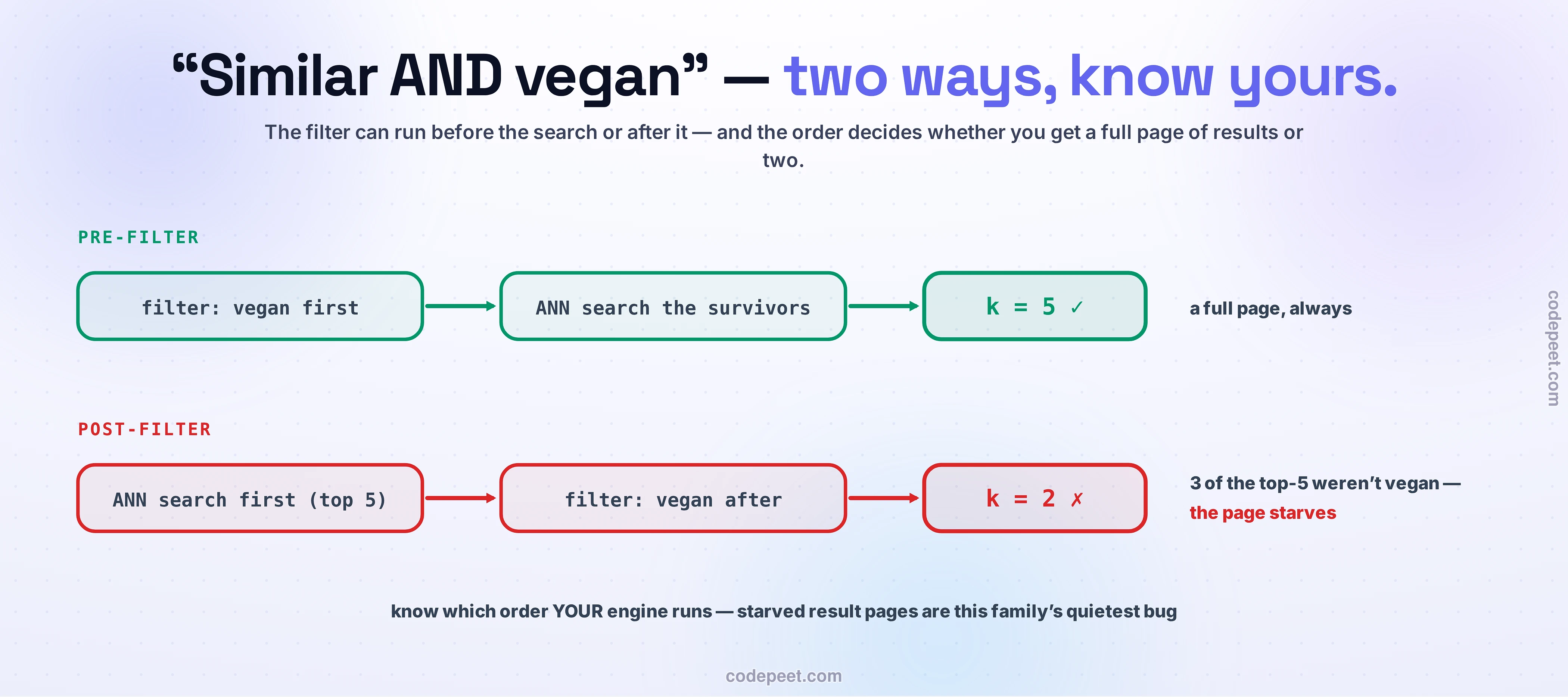
Filtered search is a real design surface. "Similar dishes, but vegan" combines vector proximity with a scalar predicate, and engines answer it two ways: pre-filter (restrict candidates to vegan first, then search — full k results, but a very selective filter can degrade the index's shortcuts) or post-filter (search first, filter after — and your k=5 can starve to 2, as you just watched). Engines differ, defaults differ; knowing which yours does is the kind of question that sorts staff engineers from tourists.

Memory is the tax. HNSW keeps its graph and the vectors in RAM — at a billion 768-dimensional float32 vectors, that's terabytes before the index overhead. Billion-scale systems reach for disk-resident designs (DiskANN-class) or shard the space — real operations, real runbooks.

Truth lives elsewhere — again. Like the search index one lesson ago, a vector index is a derived projection: embeddings are computed from source data that lives in a primary store, and they're re-computed when the embedding model changes (which, in AI-adjacent systems, is often). Same polystore posture, same rebuildable-cattle logic, same sync problem — and the same pointer: keeping derived stores honest is Outbox + CDC's story (§6). One deployment pattern, now three families deep.

Time for 2026's most interesting database argument, and this course's convergence bell rung one last time — loudly.

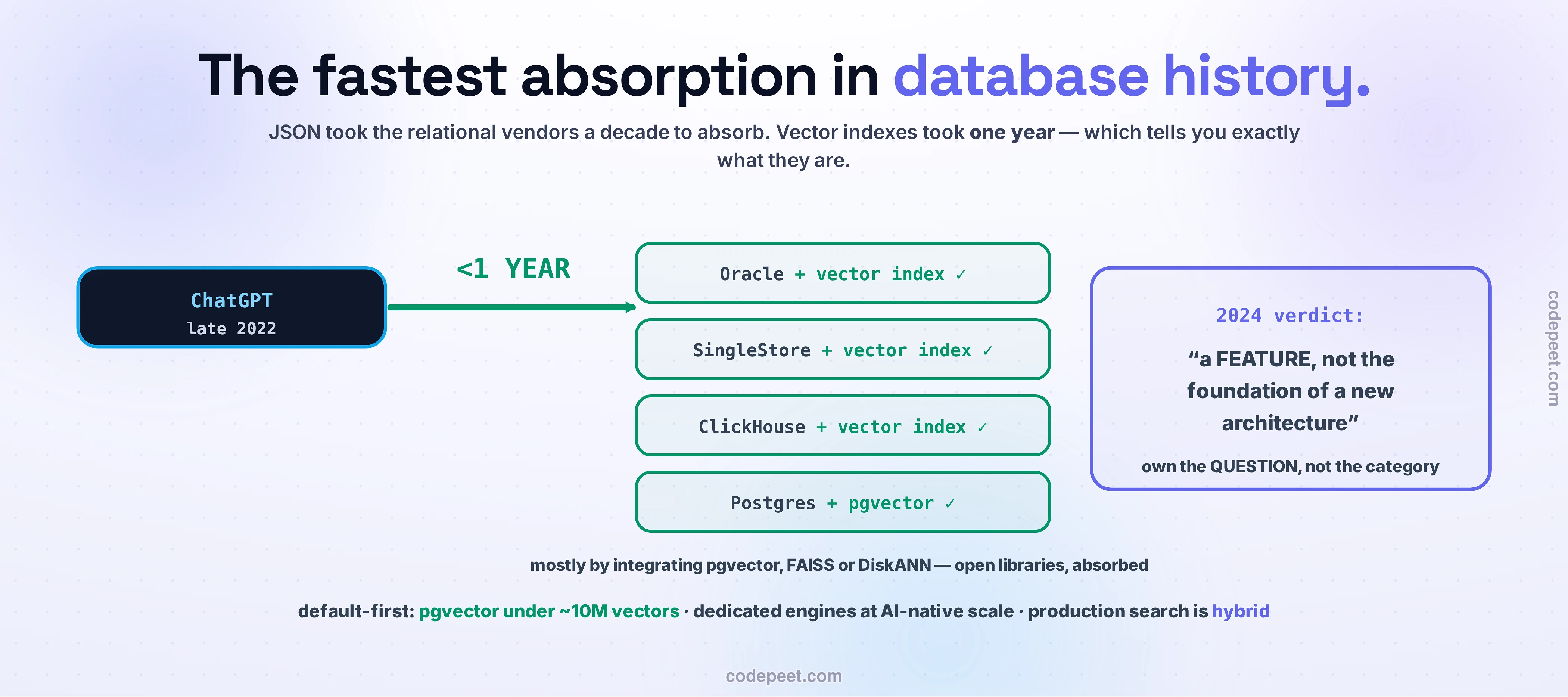
When embeddings went mainstream (late 2022), dedicated vector databases were the gold rush. Then the 2024 Stonebraker–Pavlo retrospective delivered the counter-verdict in one sentence: vector databases are "essentially document-oriented DBMSs with specialized ANN indexes — such indexes are a feature, not the foundation of a new system architecture." Their evidence was speed itself: within one year of ChatGPT, Oracle, SingleStore, Rockset, and ClickHouse all shipped vector indexes — the fastest absorption in database history (JSON support took relational vendors most of a decade) — mostly by integrating open libraries: pgvector, DiskANN, FAISS. Their prediction: dedicated vector engines will grow SQL and transactions (the document-family evolution, rerun), while every incumbent absorbs the index.

So the review-room framing writes itself, and it's the landscape lesson's rule verbatim. Default first: already on Postgres with under ~10 million vectors? pgvector is the no-brainer — headline feature at Supabase, Neon, RDS; benchmark-competitive (pgvectorscale: ~471 QPS at 99% recall). One database, one runbook, transactions with your vectors. Specialize on evidence: dedicated engines (Pinecone, Milvus, Weaviate, Qdrant) earn their keep at AI-native scale — billions of vectors, managed embedding pipelines, hybrid search, multi-tenancy — where vector search is the product.

Two closing calibrations that save real money. Hybrid beats either alone: semantic similarity finds "cozy winter soup"; lexical search finds "iPhone 15 case 2-pack" (exact tokens matter!) — production search increasingly runs both and fuses rankings; the two relevance lessons on this map are teammates. And benchmarks only compare at equal recall — the dial makes naked QPS meaningless; the first question about any vector benchmark is "at what recall@k?"

Four vector-shaped decisions from the marketplace's roadmap. Answer each; commit first.

1. "Customers who liked this dish also liked…" — 200K dishes, embeddings refreshed weekly, team already runs Postgres. Engine?
2. Your ANN index returns "similar dishes" that users rate as not similar 8% of the time. Name the two most likely dials involved.
3. "Similar dishes under ₹200 near me" — the price+geo filter matches 3% of the catalog. Pre-filter or post-filter, and why?
4. A vendor pitch says their vector DB does "12,000 QPS — 6× faster than pgvector." What's the first question you ask?

Answers. (1) pgvector — 200K ≪ 10M, one runbook, vectors next to the relational truth they derive from; a dedicated engine here is the landscape lesson's oldest mistake. (2) Recall settings (nprobe/ef_search too low → true neighbors missed) and — subtler — the embedding model itself (the DB does geometry; if the map is wrong, perfect recall retrieves perfect nonsense). Diagnose by measuring recall against an exact scan on a sample: if recall is ~100% and results still feel wrong, it's the model, and that's an AI-course problem. (3) Pre-filter — at 3% selectivity, post-filtering a top-k of similar dishes would starve to near-zero survivors; restrict to the 3% first, then search within it. (4) "At what recall@k?" — QPS without a recall number is half a spec; any ANN index can be arbitrarily fast at recall it doesn't disclose.

• "Vector databases understand meaning." The embedding model understands (and it's not in the database); the database does geometry on points it's handed. Garbage map in, confidently arranged garbage out.
• "ANN returns the nearest items." It returns most of them, probably — recall is a dial you set. You watched two true neighbors go missing at nprobe=1, with no error raised, and bought them back with the dial.
• "Every AI feature needs a vector database." The fastest absorption in DB history says otherwise: within a year, the index was a feature in every major engine. Postgres + pgvector under ~10M vectors is the default-first answer; dedicated engines earn keep at AI-native scale.
• "Vector search replaces keyword search." Different relevance: semantic (meaning — "cozy winter soup") vs lexical (exact tokens — "iPhone 15 case 2-pack"). Production search is increasingly hybrid; the map's two relevance families are teammates.
• "More dimensions = better similarity." Dimensions cost memory and latency and deepen the curse; retrieval-tuned smaller models routinely beat larger ones on the same corpus. (Choosing models: out of scope, deliberately.)
• "12,000 QPS beats 2,000 QPS." Only at equal recall@k. The dial makes naked throughput numbers meaningless — always ask for the recall.

• Meaning becomes coordinates: an embedding model places similar things near each other; the query embeds through the same model (the analyzer rule, reborn), and similarity becomes k-nearest-neighbors under a metric you choose — the metric itself reorders results.
• The first family with no exact shortcut: the curse of dimensionality kills tree indexes past ~10-D; exact NN = scan everything. The family's whole trick is ANN — a negotiated approximation where recall@k is a dial you own (IVF/nprobe: boundary misses, silent; HNSW: a navigable-small-world graph — the graph family moonlighting as an index).
• Fine print that separates production from demos: pre- vs post-filtering (post can starve below k), HNSW's RAM appetite, and the derived-index posture — truth lives elsewhere, embeddings are rebuildable projections (sync ⟶ Outbox + CDC).
• The 2024 verdict: "a feature, not a foundation" — absorbed into every major engine within a year (vs JSON's decade). Default-first: pgvector under ~10M vectors; dedicated engines at AI-native, billion-scale. Hybrid lexical+semantic is the real search answer. Benchmarks only at equal recall.
• And with that, the map is complete. Eight families, eight native questions: the value for a key · records kept correct · the whole aggregate · sorted-sparse width · relationships at depth · windows over time · relevance to words · similarity of meaning. Every one a bet frozen into a layout; every one best at exactly its question.
• Next, the axis that runs underneath all of them — why the same data lives in rows for transactions and columns for analytics: OLTP vs OLAP.