Indexes Deep-Dive

The Right Index Is Magic. The Wrong One Is Dead Weight.

Two lessons ago we said a schema models the world while indexes model the queries, and we built the B-tree that makes them fast. But we left the hard part unspoken: a B-tree on the wrong columns does nothing, a B-tree on the right columns is indistinguishable from magic, and every one you add makes every write a little slower. The craft of indexing is choosing — and it's the highest-leverage skill a backend engineer can have, because the difference is not subtle.

Here's the whole lesson in one table. It's a real 2-million-row orders table, and here's the same lookup — WHERE customer_id = 42042 — with and without the right index:

no index: a sequential scan, 49.9 ms, reading past two million rows to find twenty.
the right index: a seek, 0.083 ms.

Six hundred times faster, same query, same data. Now watch what happens as we reach for the wrong index, then the right one, then a sharper one, then a surgical one — and watch the write bill climb the whole time. By the end you'll know not just the index types — composite, covering, partial, hash — but the judgement to pick one and the honesty to count what it costs.

Scope: this is the index types and the write tax. HOW the planner decides which one to use, and the full EXPLAIN mindset, is How a Query Executes.

The leftmost-prefix rule of composite indexes, drawn with measured numbers. On the left, an index on (customer_id, created) is shown as a sorted two-column list — entries ordered first by customer_id, then by created within each customer — like a phone book sorted by last name then first. On the right, which queries can use it, measured on a real 2-million-row table: WHERE customer_id = 7 uses it as a seek, 0.083 ms; WHERE customer_id = 7 AND created > … also uses it; but WHERE created > … alone, which skips the leading column, cannot use the index at all and falls to a full scan, 127 ms. A violet panel states THE LEFTMOST-PREFIX RULE: an index is usable for any left prefix of its columns — (a), (a,b), (a,b,c) — but never for (b) alone, (c) alone, or (b,c); the leading column is the door. The amber maxim across the bottom: column order is everything — equality columns first, one range column next, sort columns last.

An Index Is a Sorted Copy of Some Columns

Strip away the vocabulary and an index is a simple thing: a sorted copy of one or more columns, each entry pointing back to its row. The B-tree lesson showed how that sorted structure lets you find a value in three page reads instead of a million. A single-column index on email keeps every email address in order with a pointer to its row, so WHERE email = 'ada@x.com' becomes a seek down the tree instead of a march through the table. That much you already have.

The interesting questions start the moment you have more than one column to filter, sort, or return — which is to say, the moment you write a real query. What does an index on two columns actually sort by? When can the database skip the table entirely? When does indexing a slice beat indexing the whole thing? Each answer is a different index type, and each one is a tool you reach for deliberately.

Composite Indexes and the Leftmost-Prefix Rule

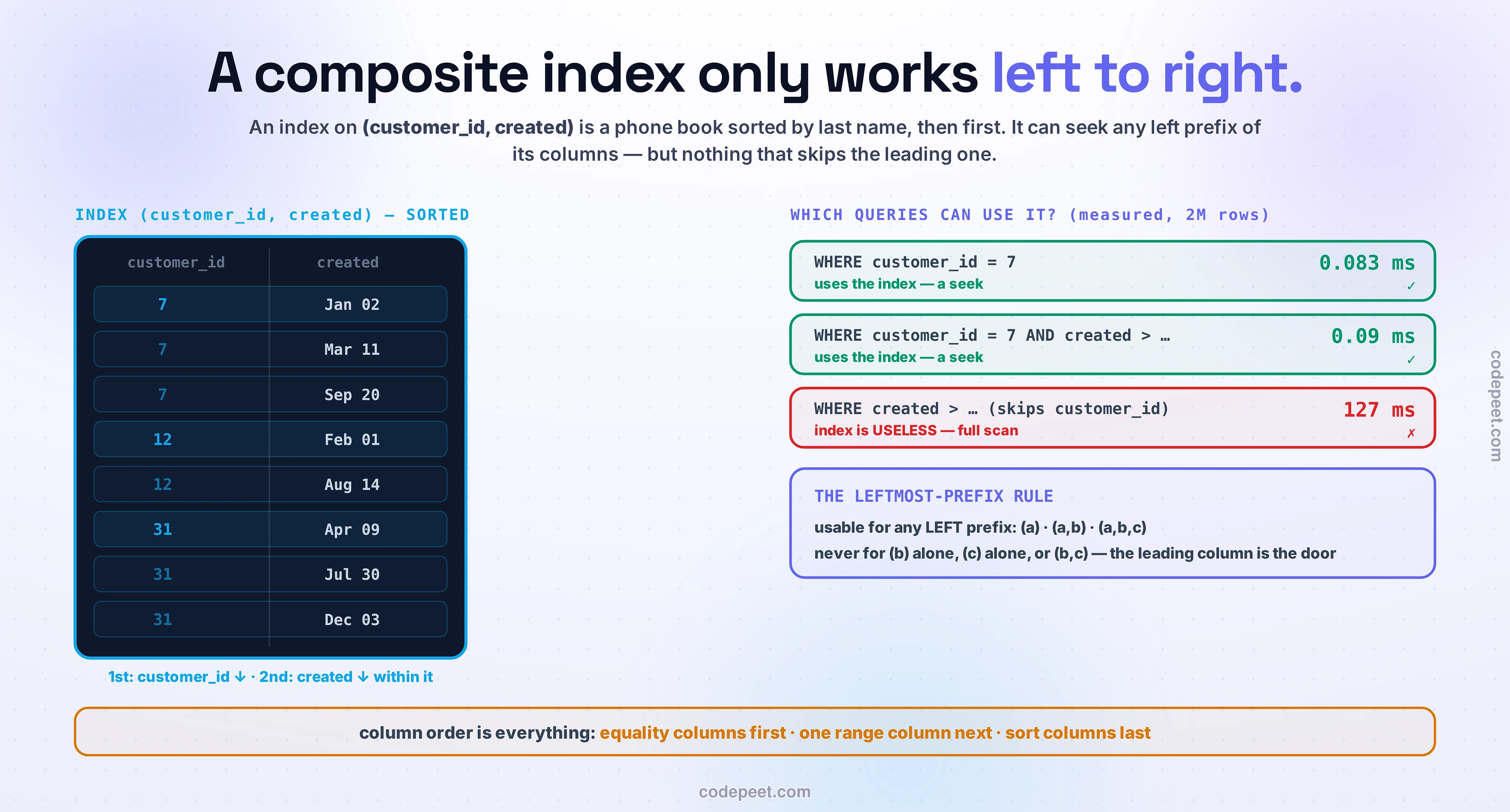
The star gotcha of indexing lives here. A (a, b, c) index is sorted by a, then b within a, then c — exactly like a phone book sorted by (last name, first name). It can seek for any LEFT PREFIX of the columns: WHERE a, WHERE a AND b, WHERE a AND b AND c — but NOT WHERE b alone, and NOT WHERE c, because b and c aren't sorted globally, only within an a. On a real 2M-row table this is stark:

-- index: (customer_id, created)
WHERE customer_id = 42042        -> Bitmap Index Scan     0.083 ms   (uses it)
WHERE created > now() - '1 day'  -> Parallel Seq Scan   127 ms       (canNOT use it)

Same index, opposite outcomes: it's lightning for the leading column and completely invisible to a query that filters only on created. Hence the column-order rule: put equality-filtered columns first, then ONE range column, then any sort columns — because a range predicate (>, BETWEEN) STOPS the usable prefix; nothing after it can be used to seek. (status, created) for WHERE status=? AND created>? is right; flip the order and the index barely helps.

Covering Indexes: Never Touch the Table

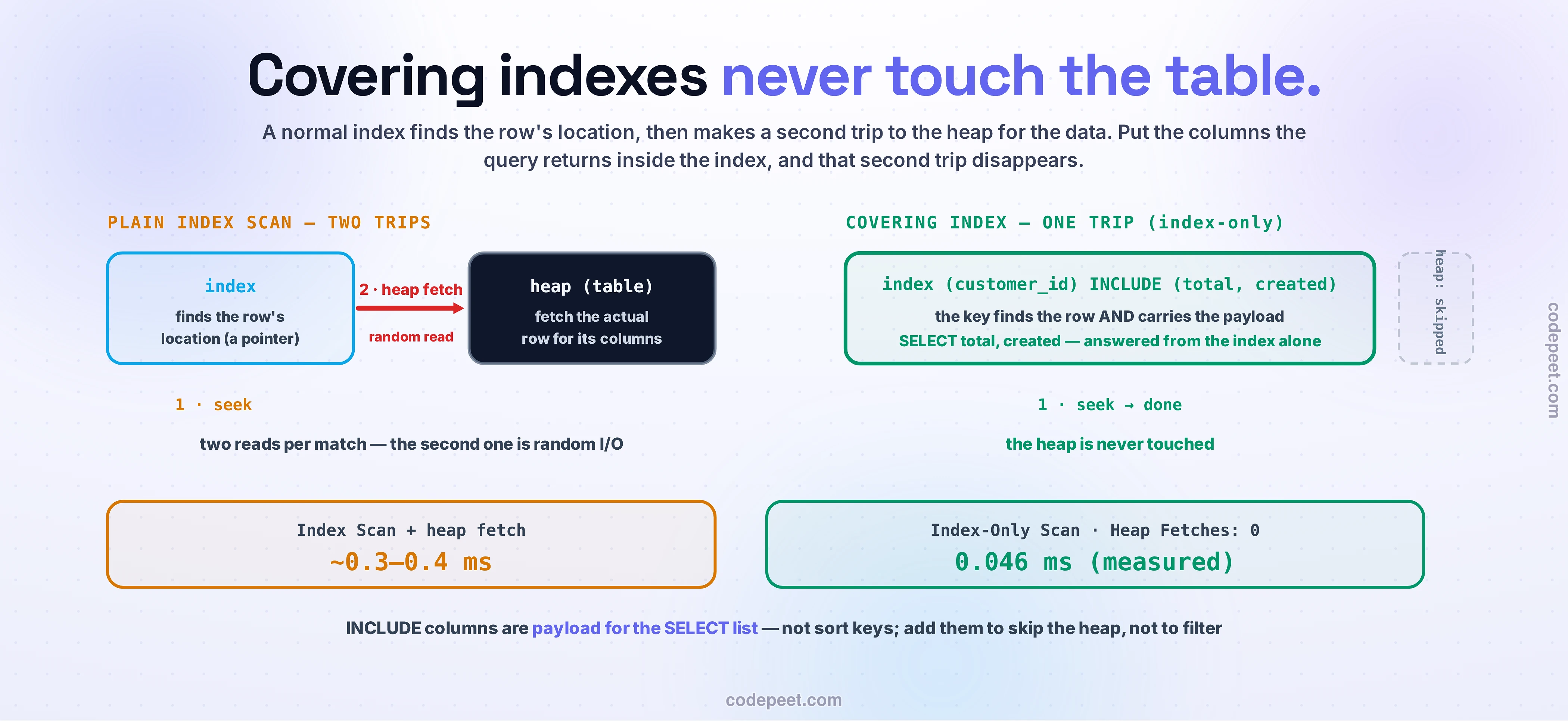
Normally a match is two steps: the index finds the row's location, then the engine fetches the actual row from the heap — a second, random read (the bookmark lookup). But if the index already CONTAINS every column the query needs, that heap fetch vanishes. Postgres calls it an index-only scan, and its INCLUDE clause (v11+) lets you bolt on payload columns that are stored-but-not-sorted:

CREATE INDEX idx_cover ON orders (customer_id) INCLUDE (total, created);
SELECT total, created FROM orders WHERE customer_id = 42042;
-- Index Only Scan ... Heap Fetches: 0     0.046 ms   (the table is never touched)

Heap Fetches: 0 is the whole point: the index answered the entire query by itself. INCLUDE is not the same as adding a column to a composite: composite columns are part of the sort order (used for WHERE and ORDER BY); INCLUDE columns are pure payload for the SELECT list. Use composite when you filter or sort on the extra column; use INCLUDE when you only need to return it.

Covering indexes drawn as two trips versus one, with measured times. On the left, a PLAIN INDEX SCAN takes two trips: a sky index box finds the row's location (step 1, a seek), then a red heap-fetch arrow makes a second, random read into the heap table for the actual row (step 2) — two reads per match, the second random I/O. On the right, a COVERING INDEX makes one trip: a green box, index on customer_id INCLUDE (total, created), where the key finds the row and carries the payload, so SELECT total, created is answered from the index alone — an index-only scan, and the heap box beside it is grayed and dashed, skipped. The measured contrast: a plain index scan plus heap fetch is about 0.3 to 0.4 ms, the index-only scan with Heap Fetches: 0 is 0.046 ms. INCLUDE columns are payload for the SELECT list, not sort keys — add them to skip the heap, not to filter.

Partial Indexes: Index Only What You Query

A partial index carries a WHERE predicate and covers only the rows that match it: CREATE INDEX … ON orders (created) WHERE status = 'pending'. When you constantly query a small hot slice of a huge table — the pending orders out of two million mostly-shipped ones — the payoff is threefold. On our real table the partial index was 2.6 MB against 13 MB for the equivalent full index — five times smaller — because it only indexes the ~18% pending rows. Smaller means faster to scan, cheaper to cache, and — the sneaky win — it's only maintained on a write when the row actually matches the predicate, so it barely taxes the shipped-order firehose at all.

Hash Indexes: Equality Only

One more type, quickly, because you'll hear it named. A hash index doesn't sort anything — it hashes each key into a bucket, like a giant hash map on disk. That makes it answer WHERE token = 'abc123' in one bucket lookup, marginally faster than a B-tree for pure exact-match traffic like session-token lookups. But hashing destroys order, so a hash index is useless for ranges, ORDER BY, or prefix LIKE — everything a B-tree does for free. That's why the B-tree is the default and the hash index is a rare specialist: reach for it only when you know every query is an exact-equality hit and you never need order. Ninety-nine times out of a hundred, you want the B-tree.

Drive It: The Query Planner Game

Here is the whole lesson as a game you play against the planner. You've got a real orders table and the five queries an app actually runs. Build indexes — pick the key columns in order, add an INCLUDE payload, mark one partial — and watch every query's plan flip live between a slow Seq Scan, a fast Index Scan, and a heap-free Index-Only Scan. The catch is the meter in the corner: every index you add raises the write cost.

Try this first: build (customer_id, created) and watch the first two queries go fast while the third — WHERE created — stubbornly stays a Seq Scan, because created isn't the leading column. That's the leftmost-prefix rule biting in real time. Fix it with its own index; turn the customer lookup into an Index-Only Scan by INCLUDE-ing the columns it returns; serve the pending query with a partial index. And keep one eye on the last query, WHERE status='shipped' — no index will ever help it, because it returns most of the table and the planner correctly refuses to use one. The goal isn't all green. It's the fewest indexes that make the queries you care about fast.

Design indexes on a real orders table and watch each query's plan flip between Seq Scan, Index Scan, and Index-Only Scan — while the write-cost meter climbs with every index you add.

The Write Tax: Every Index Has a Bill

Every index you just met has the same hidden cost, and it's time to name the bill. An index is a sorted copy — which means every insert, update, and delete has to keep that copy in sync. One index, and a write updates the table plus one more structure. Five indexes, and every single write updates six things, each with its own page splits and its own WAL records.

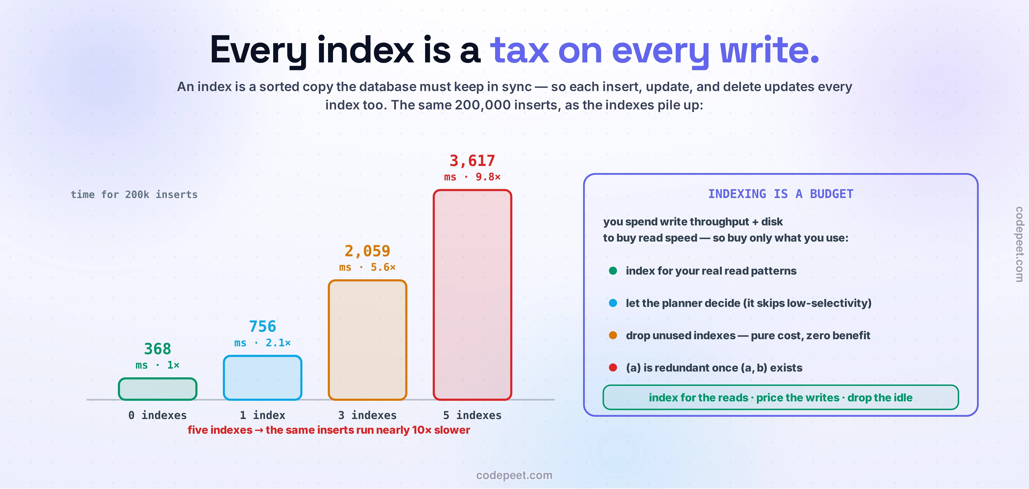
This is not a rounding error. We ran the same 200,000 inserts against the same table with a growing number of indexes:

0 indexes :   368 ms
1 index   :   756 ms   (2.1x)
3 indexes : 2,059 ms   (5.6x)
5 indexes : 3,617 ms   (9.8x)   <- the same inserts, ten times slower

Every index is a tax on write throughput, and the tax compounds. Which reframes the whole lesson: indexing isn't "add indexes until queries are fast." It's a budget. You spend write performance and disk to buy read performance, and like any budget the goal is to buy only what you'll use.

So the discipline is simple to state and easy to neglect:

Index for your real read patterns — the queries your app actually runs, not the ones it might someday. Only you know these, which is why indexing is a developer's job, not something a DBA can guess from the outside.
Let the planner decide. An index isn't used just because it exists. For a query that returns most of the table, a sequential scan beats an index plus a million random heap fetches — and the planner correctly ignores your index. We measured it: WHERE status='shipped' (82% of rows) took a 118 ms seq scan while status='pending' on a tiny slice took 0.23 ms on the index. Indexes pay only when they're selective.
Hunt the unused ones. An index nothing queries is pure cost — slower writes, wasted disk, more vacuum work, zero benefit. Postgres tracks scans per index (pg_stat_user_indexes.idx_scan); an index with zero scans over a representative window is a candidate to drop (mind the monthly-report query, and never drop one enforcing a key constraint).
Watch for redundancy. A (customer_id) index is redundant the moment a (customer_id, created) index exists — the composite already serves it via the leftmost prefix. Keep the wider one.

Index for the reads, price the writes, drop what's idle. That's the craft.

The write tax of indexes, drawn as a bar chart with the discipline beside it. Four bars show the time for the same 200,000 inserts as the index count grows: 0 indexes 368 ms (1x), 1 index 756 ms (2.1x), 3 indexes 2,059 ms (5.6x), 5 indexes 3,617 ms (9.8x) — five indexes make the same inserts run nearly ten times slower, because each index is another sorted structure every write must maintain. On the right, a violet panel titled INDEXING IS A BUDGET: you spend write throughput and disk to buy read speed, so buy only what you use — index for your real read patterns, let the planner decide (it skips low-selectivity queries), drop unused indexes which are pure cost, and note that a single-column (a) index is redundant once a composite (a, b) exists. The rule: index for the reads, price the writes, drop the idle.

🧪 Try It Yourself

Fifteen minutes and a Docker container will let you feel every claim in this lesson. These are the exact commands; the outputs are pasted from the real run.

1. Build two million rows and watch a scan become a seek.

CREATE TABLE orders (id bigint GENERATED ALWAYS AS IDENTITY PRIMARY KEY,
  customer_id int, status text, total numeric(8,2), created timestamptz);
INSERT INTO orders (customer_id, status, total, created)
  SELECT (random()*1e5)::int,
         CASE WHEN random() < 0.18 THEN 'pending' ELSE 'shipped' END,
         (random()*500)::numeric, now() - (random()*365)::int * interval '1 day'
  FROM generate_series(1, 2000000);
ANALYZE orders;

EXPLAIN (ANALYZE, COSTS OFF) SELECT * FROM orders WHERE customer_id = 42042;
--  Parallel Seq Scan ...   Execution Time: 49.9 ms

2. Add a composite index — and prove the leftmost-prefix rule.

CREATE INDEX idx_cc ON orders (customer_id, created);  ANALYZE orders;

EXPLAIN (ANALYZE, COSTS OFF) SELECT * FROM orders WHERE customer_id = 42042;
--  Bitmap Index Scan on idx_cc      0.083 ms      <- leading column: fast

EXPLAIN (ANALYZE, COSTS OFF) SELECT * FROM orders WHERE created > now() - interval '1 day';
--  Parallel Seq Scan             127 ms          <- created is NOT the leading column: index unused

3. Make it covering (Heap Fetches: 0) and a slice of it partial.

CREATE INDEX idx_cover ON orders (customer_id) INCLUDE (total, created);
VACUUM ANALYZE orders;
EXPLAIN (ANALYZE, COSTS OFF) SELECT total, created FROM orders WHERE customer_id = 42042;
--  Index Only Scan ... Heap Fetches: 0     0.046 ms

CREATE INDEX idx_pending ON orders (created) WHERE status = 'pending';
SELECT pg_size_pretty(pg_relation_size('idx_pending'));   -- 2608 kB  (vs 13 MB for a full one)

4. Predict, then measure the write tax. Before you run this, guess how much slower 200k inserts get with five indexes versus none:

CREATE TABLE wt (id bigint, customer_id int, status text, total numeric, created timestamptz);
\timing on
-- time this INSERT with 0 indexes, then add indexes and TRUNCATE + re-run:
INSERT INTO wt SELECT g,(random()*1e5)::int,'shipped',(random()*500)::numeric,now()
  FROM generate_series(1,200000) g;
--  0 idx: 368 ms   1 idx: 756 ms   3 idx: 2059 ms   5 idx: 3617 ms

Clean up with docker rm -f <container> when you're done.

Mental-Model Corrections

"Just index everything — more indexes, faster database." Faster reads on the queries that match, slower everything else. Each index taxes every write (we clocked ~10× at five indexes), eats disk, and adds vacuum load; an index no query uses is pure cost. Index for the read patterns you actually have.
"More columns in one index means it covers more queries." The opposite trap. The leftmost-prefix rule means (a, b, c) does nothing for WHERE b or WHERE c alone — only for left prefixes. A well-ordered two-column index beats a carelessly ordered five-column one. Order is the whole game.
"If I create the index, my query will use it." Only if the planner decides it's cheaper. For a query returning a big fraction of the table, a sequential scan beats an index plus a storm of random heap fetches, and the planner correctly skips your index (shipped: 118 ms seq scan; pending: 0.23 ms index — same column, opposite call). Indexes reward selectivity.
"A covering index is just a composite index." No — INCLUDE columns are non-searchable payload carried for the SELECT list; composite columns are the searchable, sorted key. You add a composite column to filter or sort on it; you INCLUDE a column only to return it without a heap fetch.
"Indexes only speed up WHERE clauses." They also serve ORDER BY for free (the leaves are already sorted) and answer whole queries by themselves via index-only scans. An index matches the shape of a query — its filter, its sort, and its returned columns — not just its filter.

Key Takeaways

An index is a sorted copy of some columns with a pointer to each row — the same B-tree, aimed at the queries you actually run.
Composite indexes obey the leftmost-prefix rule: (a, b, c) serves WHERE a, a AND b, a AND b AND c — never b alone. Order the columns equality-first, one range next, sort columns last. (Measured: the leading column ran 0.083 ms; the same index was useless for a non-leading filter, 127 ms.)
Covering indexes carry the query's columns as INCLUDE payload so the answer comes from the index alone — an index-only scan, Heap Fetches: 0.
Partial indexes index only the rows you query (2.6 MB vs 13 MB), and only maintain them on writes. Hash indexes do equality-only and are a rare specialist.
Every index is a write tax — the same inserts ran ~10× slower with five indexes. Index for reads, count the writes, and let the planner decide (it ignores an index that isn't selective).

You now have the storage engine whole: how a write travels, how B-trees and LSMs store it, how the WAL protects it, and how indexes aim it. One question keeps recurring under all of it — how does the planner actually choose which index, which join, which scan? That's the finale of this section: How a Query Executes.