LSM Trees & SSTables

Last lesson ended on a fork. A B-tree is a magnificent reader, but it pays for it on writes: every change rewrites a whole page in place, and random keys scatter that cost across the disk. We asked: what if your workload is the opposite — a firehose of writes you'll rarely read back?

That workload is everywhere. Discord ingests trillions of chat messages; a fleet of sensors emits a reading every second; a metrics pipeline never stops. These systems write constantly and, mostly, never look back. Hand that to a B-tree and it drowns in page rewrites. So the engines built for it — Cassandra and ScyllaDB (the wide-column family from earlier), RocksDB, LevelDB, HBase — all reach for a completely different structure that makes the opposite bet. It has one governing rule, and everything else in this lesson falls out of it.

Scope: this is the storage engine — memtable, SSTable, compaction, bloom filters. The durability log that backs the memtable is WAL & Durability: Why Committed Data Survives; hash and secondary indexes are Indexes Deep-Dive.

Here is the rule the whole structure is built to obey: never modify data on disk — only append. A B-tree seeks to a page and rewrites it; that random in-place write is the expensive thing. An LSM tree simply refuses to do it. Existing files are never touched.

So where does a write go? Two places, both cheap. First it's appended to a commit log on disk — a plain append-only file that survives a crash (its full machinery is next lesson's subject). Then it's inserted into the memtable: an in-memory structure that keeps keys sorted as they arrive — a skip list or balanced tree. That's the entire write path. An in-memory insert plus a sequential log append, both measured in microseconds, and the client hears done. The disk never once did a random write. This is why an LSM absorbs writes a B-tree would choke on — but it should nag at you: if we keep the data in memory and only ever append, how does anything permanent get organized?

When the memtable fills, the engine flushes it: writes the whole thing to disk, in one sequential pass, as a single file called an SSTable — a Sorted String Table. Because the memtable was already sorted, there's no sort step; it just streams out. And the file is immutable — once written, never modified, ever. A fresh memtable takes over for new writes.

You can watch this happen on a real Cassandra. One flush of a messages table produced a little family of sibling files, born together and never edited again:

That immutability has a consequence you can see on disk. If you update a key, the new value lands in the new memtable and eventually a new SSTable — the old value still sits untouched in the old one. So the SSTables pile up. Flush after flush after flush, each a sorted snapshot of whatever was in memory at the time. Measured, with compaction paused: five flushes left five Data.db files on disk — the count climbed 1 → 2 → 3 → 4 → 5, one per flush. The disk is now a stack of immutable, sorted files, newest on top. Fast to write to. But think about reading.

Your key could be in the memtable, or the newest SSTable, or the one before it, or the oldest — you don't know. So a read checks the memtable, then each SSTable newest to oldest, until it finds the key. With five files on disk that's up to five lookups for one read. This is read amplification, and it's the price the LSM pays for its cheap writes: reading got harder so writing could get easy.

Two rescuers make it bearable. Each SSTable is sorted and ships with a sparse index, so within a file you binary-search rather than scan. And each SSTable carries a Bloom filter — a tiny probabilistic structure (24 bytes on our table) that answers one question in memory: is this key definitely NOT in this file? If the filter says no, the read skips that file entirely, never touching the disk. A Bloom filter can be wrong in exactly one direction — it may say "maybe present" for a key that's absent (a false positive, a wasted lookup), but it will never say "absent" for a key that's there. So it can safely eliminate files, and that's what makes reading a stack of SSTables fast enough to ship. Without Bloom filters, every read would frisk every file.

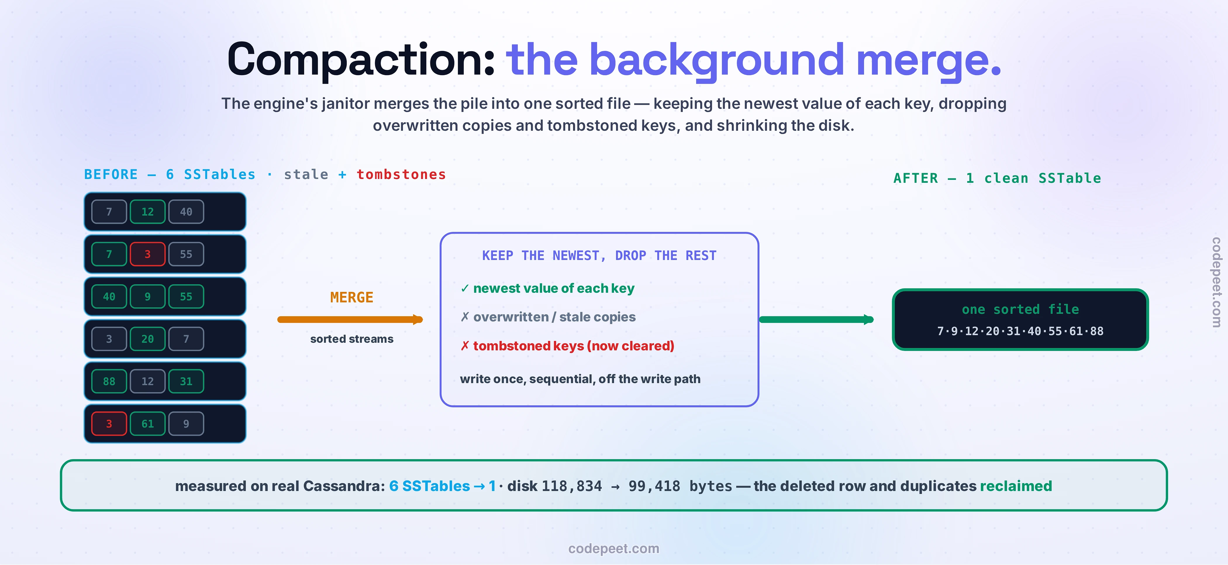
A pile that only grows is a disease with an obvious end: reads get slower forever, disk fills with stale versions, and — the strangest part — deleted data never actually leaves. Because you can't erase from an immutable file, a delete can't remove anything. It writes a marker called a tombstone: a little record that says "this key is gone as of now." A read that hits the tombstone before any older value reports the key as deleted. Which means the counter-intuitive truth of this whole structure: a delete is a write. It makes the data bigger. We measured it — one DELETE plus a flush took the SSTable count from 5 to 6.

The cure for all of it is compaction — the engine's background janitor, and the heart of the design. Compaction picks several SSTables, reads them together, and merges their sorted key streams (cheap, because they're all already sorted). For each key it keeps only the newest version and drops the rest — overwritten values, and any key whose newest record is a tombstone. The merged result is written out as one new, consolidated SSTable, and the old inputs are deleted. On the real table, nodetool compact collapsed 6 SSTables into 1 and shrank Space used from 118,834 to 99,418 bytes — the deleted row and the duplicate cells finally reclaimed.

Notice what compaction is: it rewrites data that was already on disk, sometimes many times over its life. That's write amplification — the LSM's real cost — but it's paid in the background, in sequential passes, off the write path the user waits on. The engine trades a predictable background chore for a blazing-fast foreground. How aggressively it runs that chore is the one big knob, and it's what you'll turn next.

Everything so far — the memtable, the flush, the pile, the merge, the two strategies — is one machine, and here it is to drive. Turn up the write rate and pour writes in: watch the memtable fill, flush to an L0 SSTable, and compaction pull the pile up into levels in real time. Read a key and watch the bloom filters skip the files it can't be in. The three amplification meters — write, read, space — update with every action.

Try this first: write a few bursts on leveled, then flip to tiered and watch the same data resettle. Leveled does more merge work to keep tidy levels (its write amplification climbs); tiered merges lazily and lets overlapping runs pile up (read and space pay instead). You're not reading about the triangle anymore — you're moving it, one corner at a time, and feeling the other two push back.

"Merge some SSTables" leaves one question open: which ones, and how often? The two classic answers are worth knowing by name, because they're the same knob set to opposite extremes.

Size-tiered (STCS) — Cassandra's default — waits until it has a handful of similarly-sized SSTables (typically four) and merges them into one bigger one, which joins the next size tier up. It's lazy: few merges, so low write amplification. But many overlapping tables coexist, so reads probe more files and old copies linger — higher read and space amplification (a big merge can transiently need ~2× the disk).

Leveled (LCS) — RocksDB's default — organizes SSTables into levels L0, L1, L2…, each about ten times larger than the one above it. Crucially, within any level below L0 the SSTables hold non-overlapping key ranges, so a read touches at most one SSTable per level. That keeps read and space amplification low — but maintaining those clean levels means merging far more often, pushing one file down into ten it overlaps, so write amplification is high (worst case, a byte can be rewritten 50+ times on its way to the bottom level).

There's no free choice here — the two strategies just pick different corners of the same triangle, which is the whole point of the next section.

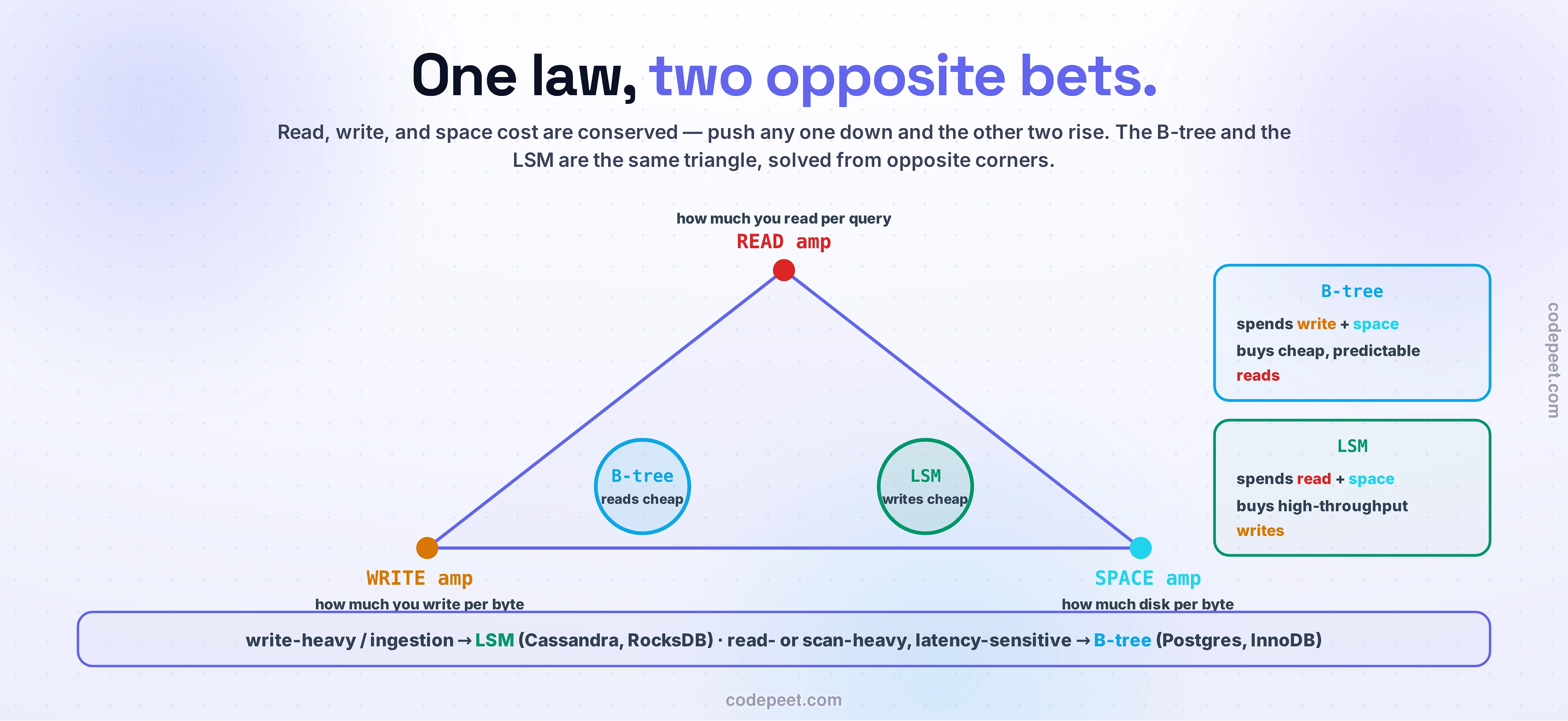
Last lesson named a law and promised its other half. Here it is. Every storage engine juggles three costs — read amplification (how much you read to answer a query), write amplification (how much you write to store a byte), and space amplification (how much disk a byte occupies). They're conserved: you can drive any one toward zero only by pushing the other two up. There is no engine that wins all three.

A B-tree spends write and space to buy cheap, predictable reads — one seek to a row, latency you can set your watch by, because there's no big background job to hiccup. An LSM makes the mirror bet: it spends read and space to buy cheap writes. Sequential appends and memory-speed commits give it write throughput a B-tree can't touch — but reads probe multiple files, and compaction runs in the background, occasionally spiking latency when it falls behind. That last point is a real failure mode, not a footnote: under a sustained write flood, if the newest level (L0) piles up faster than compaction can drain it, engines like RocksDB and Cassandra deliberately stall incoming writes to let the janitor catch up. The write-optimized engine, pushed hard enough, throttles writes. And those tombstones don't just cost space — in a replicated store, one dropped too early (before every replica saw the delete) lets deleted data resurrect, which is why Cassandra keeps tombstones for a gc_grace_period of ten days by default.

So the choice between them isn't "which is faster" — it's which amplification can your workload afford. A firehose of writes you rarely read back — event logs, metrics, chat messages, sensor streams — flatters the LSM. A read- or scan-heavy, latency-sensitive, transactional workload flatters the B-tree. Most of the databases you'll pick up have already chosen: Postgres and MySQL/InnoDB are B-trees; Cassandra, ScyllaDB, RocksDB, and the storage under many time-series and streaming systems are LSMs. Knowing why each chose is the difference between memorizing a landscape and reading it — and it's exactly the decision the section checkpoint will hand you, three times, with three different read/write mixes.

You can watch every claim in this lesson on a real LSM engine in about fifteen minutes. This is Cassandra — the wide-column database from earlier — in Docker; the outputs are pasted from the real run.

1. Start Cassandra and make a messages table.

2. Freeze the janitor, then watch the pile grow. Turn off auto-compaction so you can see each flush land, then insert a batch and flush it — five times.

3. Prove a delete is a write. Delete one row, flush, and count again:

4. Predict, then compact. Before you run this, write down how many SSTables you'll have afterward and whether Space used will go up or down. Then merge them:

Six files became one, and the disk got smaller even though you never ran a VACUUM or a DELETE-then-OPTIMIZE — compaction did it as a side effect of merging. Clean up with docker rm -f lsm.

• "LSM trees are just faster than B-trees." They're write-optimized, not faster-at-everything. Writes are cheap because they're sequential; reads can be slower (probe several SSTables) and compaction can spike latency. It's the opposite bet, not a free upgrade — pick it for the workload, not the benchmark headline.
• "Deleting frees space." A delete writes a tombstone — it makes the data bigger and can slow reads until compaction clears it (you measured the file count going 5 → 6). Space comes back later, when the janitor runs, not when you hit delete.
• "The SSTable is the write-ahead log." Two different files with two different jobs. The commit log (next lesson) is an append-only durability journal, replayed after a crash. An SSTable is a sorted, immutable data file flushed from the memtable. One protects the write; the other stores it.
• "Compaction is a nice-to-have you can tune off." It is the engine. Without it, reads scan an ever-growing pile, disk never reclaims stale versions, and tombstones never clear — performance decays to unusable. You tune how it runs, never whether.
• "A Bloom filter tells you the key is there." It only ever says definitely not here or maybe here. A false positive costs one wasted lookup; it never returns a wrong answer. That one-sided guarantee is exactly what makes it safe to skip files with.

• One rule drives everything: never modify data on disk, only append. A write hits the commit log plus an in-memory sorted memtable — memory-speed, no random disk writes.
• The memtable flushes to an immutable, sorted SSTable; new writes make new SSTables, so they pile up (measured 1 → 5, one per flush). A delete writes a tombstone — it adds a file, it doesn't erase one.
• Reads probe the memtable and SSTables newest-to-oldest (read amplification), rescued by per-file sparse indexes and Bloom filters that skip files a key can't be in.
• Compaction merges SSTables, keeps the newest value per key, drops overwritten and tombstoned data, and shrinks the disk (measured 6 files → 1, 118,834 → 99,418 bytes). It's the engine's write-amplification cost, paid sequentially in the background.
• Size-tiered vs leveled compaction picks opposite corners of the read/write/space triangle — lazy-and-write-cheap versus tidy-and-read-cheap.
• The LSM is the write-optimized mirror of the B-tree: it spends read and space to buy cheap writes, so it wins write-heavy, ingestion-shaped workloads (Cassandra, ScyllaDB, RocksDB) and loses to the B-tree on read-heavy, latency-sensitive ones.

The commit log we kept waving at — the thing that makes a memory-first, append-only engine safe to trust with your data through a crash — is the whole subject of the next lesson: WAL & Durability: Why Committed Data Survives.