Graph Databases

The marketplace's fraud team has a problem that none of your five families can touch. A stolen card was used on account 4471. That account shares a delivery device with three other accounts. One of those shares a saved address with a fourth, which funded a brand-new "restaurant" that only ever sells to… the first account. How deep does the ring go?

You don't know until you walk it. That's the sentence that defines this lesson. Every question you've asked a database so far had a known shape: a key, a page of an aggregate, a sorted slice. This one is different in kind — follow the connections, wherever and however deep they lead. Fraud rings, "people you may know," supply-chain contamination, money laundering, dependency resolution: the question's DEPTH is a variable, discovered while answering it.

The relational lesson taught you that joins recombine facts at read time — and that they're the fair price of honest storage. This lesson asks the uncomfortable follow-up: what happens when recombination-at-depth is the whole workload? The answer splits into beautiful physics, one genuinely great trick, and the most honest "it depends" on the entire database map.

In this lesson: the property-graph model (your whiteboard, stored verbatim), the cost algebra of joins-at-depth vs pointer-hops (you'll put a meter on both), the supernode that humbles every engine, why graphs shard worse than anything else you'll meet — and production's split verdict, where LinkedIn built a bespoke graph engine and Facebook serves Earth's biggest graph off MySQL.

Scope: graph analytics (PageRank, community detection over the whole graph) gets one honest paragraph, not a curriculum; collaborative/replicated state is C3's CRDTs; social-feed fan-out is Interview Mastery's Fan-out: Feeds & Timelines. This lesson is the family and its one big trick.

Every data model so far asked you to translate the whiteboard: entities into tables, aggregates into documents, access patterns into partition keys. The property-graph model is the first one that doesn't. What you draw is what's stored: nodes (circles) and edges (arrows), both typed, both carrying properties.

Here's the fraud neighborhood in Cypher — the query language Neo4j popularized, whose style fed the new SQL/PGQ and GQL standards:

Read the middle of that pattern: *1..4. Between one and four hops, through any mix of those edge types. That's variable-depth traversal expressed as naturally as a WHERE clause — and it's the shape SQL has always been awkward at, because in SQL each hop is another self-join you must write out (or a recursive CTE you must be somewhat brave about).

Two structural notes before the physics. First: relationships here are data, not schema — an edge is a stored fact you insert and delete like a row, not a foreign-key rule declared once (that difference is why edges can carry properties: since: 2024, weight: 0.8, flagged: true). Second: the model is called a property graph to distinguish it from RDF/triple stores, the semantic-web branch of the family — real, standards-rich, and one line is all it needs here.

Strip away the marketing and the graph family has exactly one big trick. It's a good one.

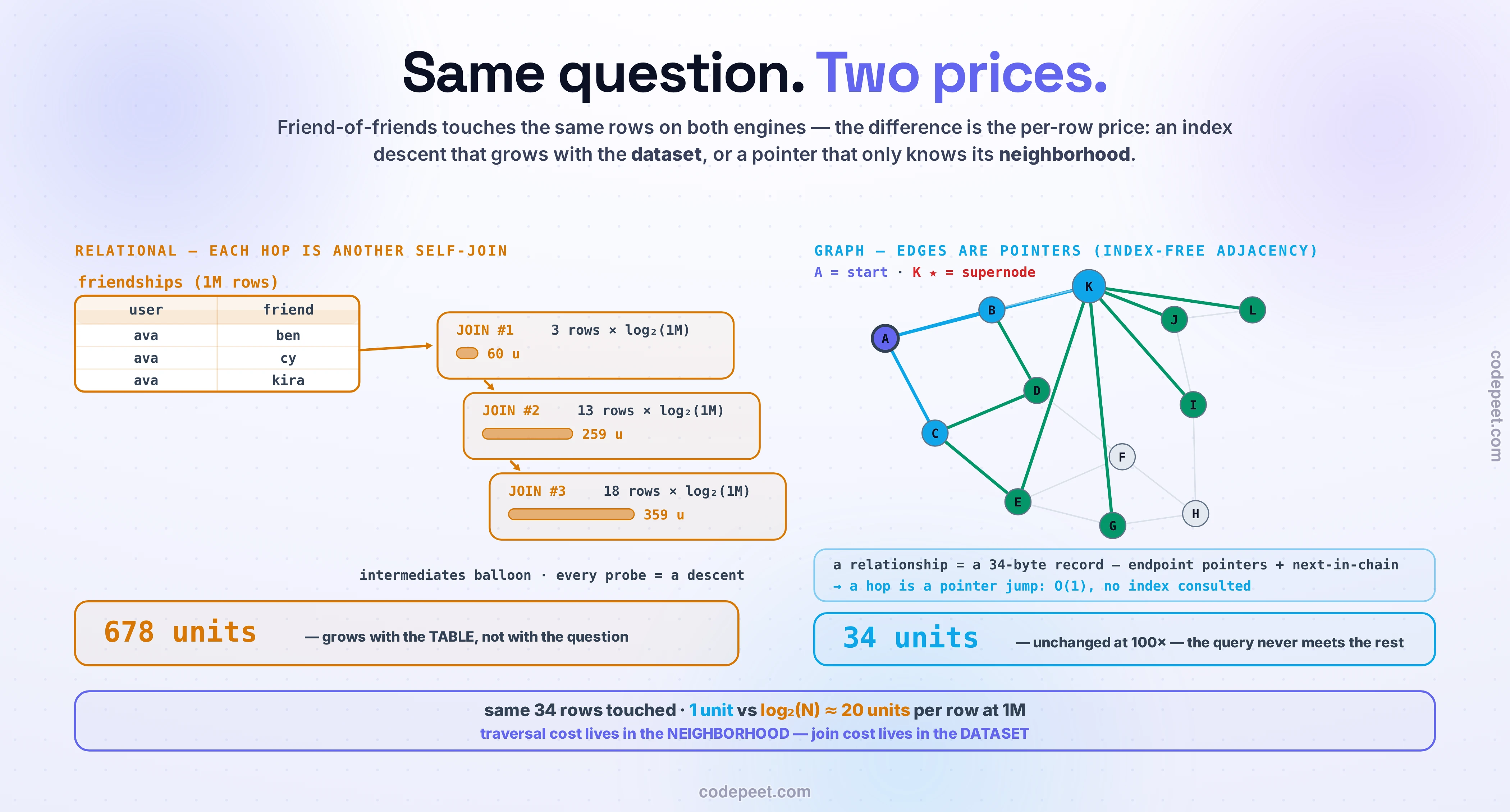
Ask relational Postgres for friends-of-friends and here's what each hop costs: for every person in the current frontier, an index probe into the friendships table — a B-tree descent, roughly log₂(N) page-touches — to find their rows. The rows found become the next frontier, and you pay again. Two things grow on you at once: the frontier (3 friends → 13 candidates → 18 more) and the per-probe price, because that log₂(N) is a function of how big the whole table is. A million friendships? Each probe walks a ~20-level descent. The query's cost is coupled to the size of data it will never touch.

A native graph store makes one radical storage decision instead: the edge IS a pointer. In Neo4j's on-disk format, a node is a fixed 15-byte record and a relationship a fixed 34-byte record holding direct offsets to its two endpoint nodes and to the next relationship in each of their chains. Fixed sizes mean an ID converts to a disk offset by arithmetic. Following an edge is a pointer jump — O(1) per hop, no index consulted, ever. They call it index-free adjacency, and its consequence is the sentence worth memorizing:

Traversal cost is proportional to the neighborhood you touch — not to how much data exists. Grow the database a hundredfold; Ava's friends-of-friends costs exactly what it cost before, because the query never meets the rest of the graph.

So the honest algebra, which the widget below turns into meters: both engines touch the same rows. The difference is the per-row price — a pointer (call it 1 unit) versus an index descent (log₂(N) units, ≈20 at a million rows). Small at depth 1. Compounding, decisive, at depth 3 on a big table. That asymmetry — neighborhood versus dataset — is the entire reason this family exists.

Twelve people, twenty friendships, one celebrity. The same question runs both ways, with the work counted honestly.

Run this arc: click Ava at 1 hop and read the verdict — SQL is fine, and the lesson says so out loud. Go to 3 hops on the 1M-row table — watch the JOIN chips stack and the ×20 gap open. Flip to 10K rows — exactly one meter moves, and that's index-free adjacency in a single gesture. Then click Kira ★, the supernode, and watch both engines pay. Finish with "count users by city" — the graph engine's trick buys nothing there, and knowing that is half of owning this family.

Two hard truths keep this family honest — one you just clicked, one that shapes the entire market.

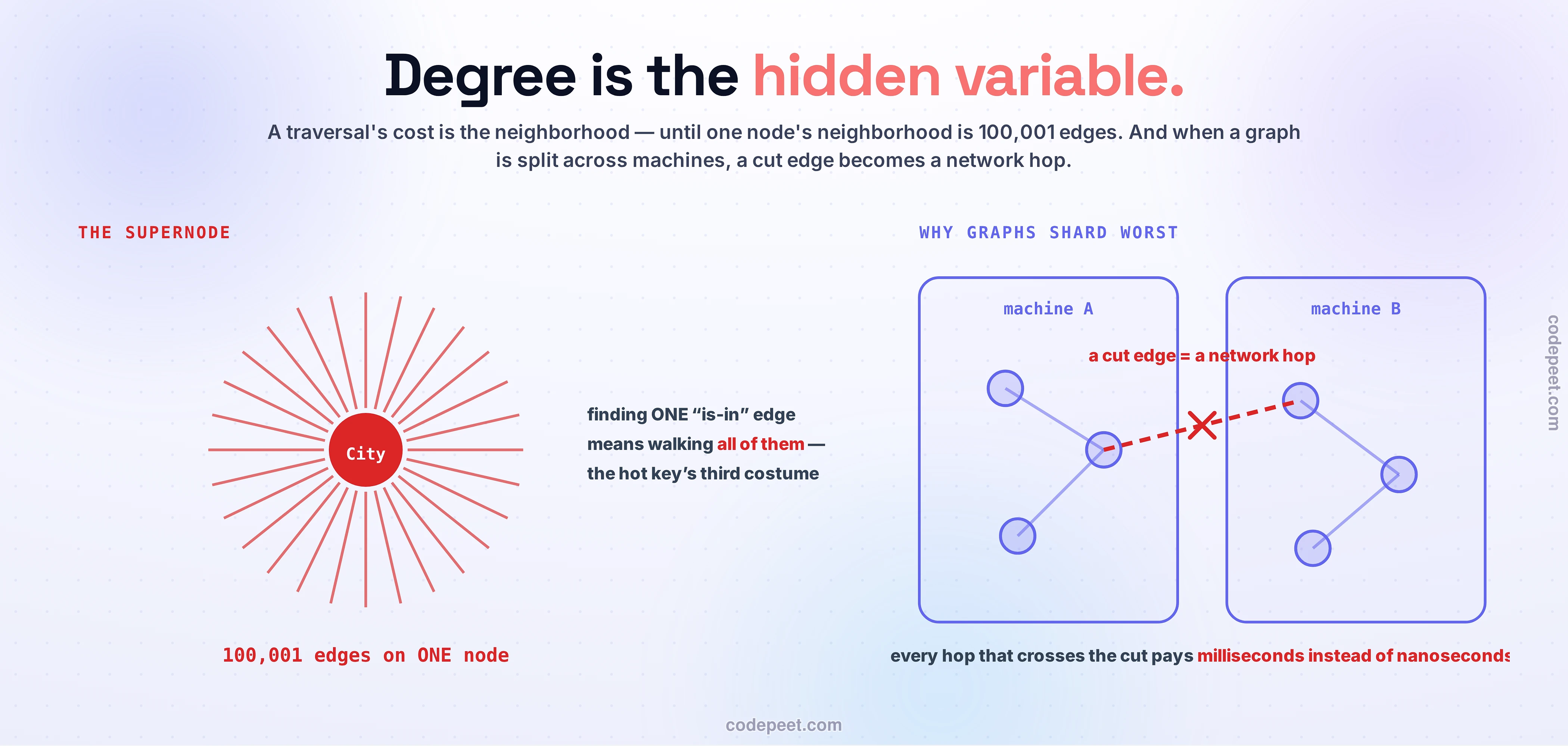
The supernode. "O(1) per hop" quietly assumed hops land on ordinary nodes. But a celebrity followed by ten million people is ten million relationship records chained together — and a traversal arriving there must walk the chain. The canonical horror story from Neo4j practice: a City node with 100,001 relationships, scanned end to end to find the one IS_IN edge a query wanted. Degree is the hidden variable in every traversal bound — and you should be having déjà vu, because this is the hot key in its third costume: one KV key melting one shard, one wide-column partition taking a viral channel, one graph node with the world attached to it. The cures rhyme too: split the hub, separate edges by type, cache what's hot. Skewed popularity follows your data through every model on this map.

Sharding. Here's the deeper structural fact, and it explains the family's whole market position. Hash-sharding gave KV and wide-column stores effortless scale-out because keys never reference each other — any key can live anywhere. A graph is the opposite: it is nothing but references. Cut it across machines and every edge crossing the cut turns a 1-unit pointer-jump into a network round-trip — five or six orders of magnitude slower — and social graphs, being power-law-shaped, have no clean place to cut. This is why the 2024 Stonebraker–Pavlo retrospective concludes that distributed graph processing "rarely outperforms single-node" implementations, why LinkedIn's LIquid is an in-memory design, and why nobody sells you "Cassandra for graphs." The family's scale story is tall machines and replicas, not fleets.

(For whole-graph analytics — PageRank, communities, centrality — the same logic ends somewhere specific: compress the graph into one big machine's memory and run there. A one-paragraph fact worth exactly one paragraph.)

Now the section that separates this lesson from every vendor page: the two biggest graph workloads on Earth chose opposite engines, and both were right.

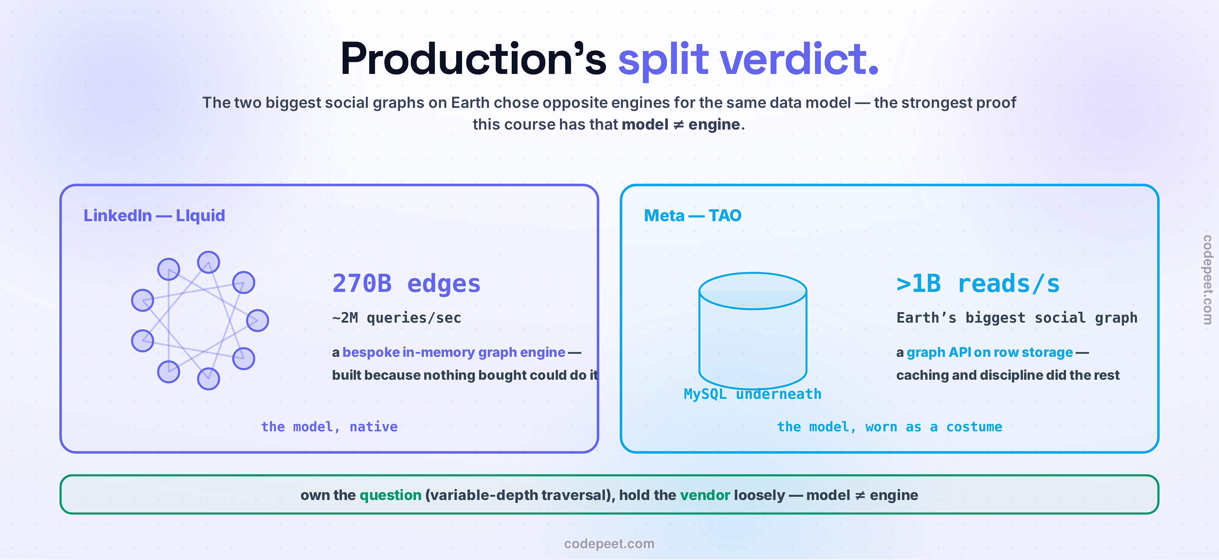
LinkedIn built the graph engine. "People you may know," second-degree search, shared-connection counts — LinkedIn's whole product is variable-depth traversal, latency-sensitive, at social scale. Their answer is LIquid: a bespoke, in-memory graph database holding 270 billion edges and serving around 2 million queries per second. When variable-depth traversal is your primary workload, you end up with a real graph engine — even if you have to build it.

Facebook didn't. Meta's social graph — the largest on Earth — is served by TAO at over a billion reads per second (96.4% cache-hit)… and TAO is a graph-shaped API and cache sitting on MySQL. The workload is graph; the store is relational; the graph-ness lives in the access layer. Why does it work? Look at the actual queries: friends-of, likes-of, comments-on — overwhelmingly depth-1 association lists, cache-friendly and key-addressable. Facebook's workload didn't need deep traversal at read time, so it didn't need a graph engine underneath.

Hold both up together and you get the cleanest statement yet of a distinction this course keeps sharpening: the model and the engine are separate decisions. Both companies think in graphs. They store according to their query depth. And the convergence pincer is closing from the relational shore too: SQL:2023 standardized property-graph queries (SQL/PGQ), and DuckDB's implementation already beats a leading native graph database by up to 10× on traversal benchmarks — the 2024 retrospective expects OLTP graph workloads to be "largely served by RDBMSs." The families keep teaching us the same thing: identities, not walls.

The decision, stated for a design review.

Reach for a graph engine when variable-depth or unbounded-depth traversal is a primary, latency-sensitive workload. Fraud rings ("how far does this spread?"), recommendation paths, dependency and impact analysis, network topology, knowledge navigation. The tell is in the question's grammar: if it contains "…of…of…" an unknown number of times, or "any path between," the family earns its keep.

Don't reach for it because your data "has relationships." All data has relationships — the relational family was named for them. Fixed-depth questions are joins: "orders with their items" (depth 1), "my friends" (depth 1), even "friends of friends" as a nightly batch (depth 2, and nobody's waiting). Modern Postgres handles moderate traversal with recursive CTEs and, increasingly, PGQ. The graph engine is a second database with its own runbook — the polyglot bill from One Size Fits None applies in full, and it's paid for by query shape, not by enthusiasm.

And calibrate with production's verdict. If your traversal is real but shallow and read-heavy — TAO's shape — a cache-fronted relational store may serve it at a billion reads a second. If it's deep, variable, and the product itself — LIquid's shape — you're in genuine graph territory. Between those poles, start relational, measure the depth of the questions users actually ask, and let the meter you drove in the widget make the call. The full checklist, as always: SQL vs NoSQL: The Decision Rubric.

Four workloads from the marketplace's roadmap. For each: graph engine, or something you already have — and one sentence of why. Commit before scrolling.

1. "Show each order with its restaurant and courier" — three entities, every order page.
2. Fraud: "given a flagged card, find every account reachable through shared devices, cards, or addresses — however many steps it takes" — must run in <200 ms at checkout.
3. "Customers also ordered…" — precomputed nightly from co-purchase pairs.
4. "Which delivery zones become unreachable if this depot closes?" — road segments and depots as a network, planners ask it interactively with what-if edits.

Answers. (1) A join — fixed depth 1, exactly what your relational store does natively; putting this in a graph engine is buying a scalpel to butter toast. (2) Graph engine — variable-depth (*1..N), latency-bound, primary workload: this is the textbook case, almost word for word LIquid-shaped. (3) Neither engine matters — depth-2, run as a nightly batch: a self-join at 3 a.m. is fine, and the results land in a KV cache for serving (families composing, exactly as the landscape lesson promised). (4) Graph — reachability under edge-removal is pathfinding with what-ifs, interactive: recursive CTEs will technically answer it and planners will technically stop using your tool. Notice the pattern in all four: the decision never mentioned what the data is — only the shape and depth of the question.

• "My data has relationships, so I need a graph database." All data has relationships; the relational family is literally named for them. The graph tell is variable or unbounded traversal depth as a primary workload — foreign keys are not a graph workload.
• "SQL can't do graphs." Node/Edge tables, recursive CTEs, and now SQL/PGQ (DuckDB: up to 10× a native graph DB) say otherwise. The honest claim is narrower and still real: at depth on large tables, join work scales with the dataset while traversal scales with the neighborhood.
• "Traversal is O(1), full stop." Per hop, per ordinary node. A supernode's chain must still be walked — 100,001 relationships to find one. Degree is the hidden variable; skew is the same enemy it was in the KV and wide-column lessons.
• "Graph databases are fast at everything graph-shaped." Aggregates, scans, and whole-graph analytics gain nothing from pointer-hops — you drove this one ("count users by city": ×1). The trick is per-hop cost. That's it, and that's enough.
• "It'll scale out like my other NoSQL stores." Worst-sharding family on the map: every cross-machine edge turns a pointer into a network hop, and power-law graphs offer no clean cuts. Big graphs live in big memory (LIquid) or behind relational farms (TAO).
• "Facebook uses a graph database, so we should." Facebook uses a graph model over MySQL, because its reads are shallow association lists. LinkedIn built a real graph engine, because its reads are deep. Same conclusion from both: choose the model for your questions, the engine for your query depth.

• The property graph stores the whiteboard verbatim — typed nodes and edges, both with properties; edges are data, not schema. Its native question: follow the connections, however deep — depth as a variable, discovered while answering (fraud rings, PYMK, reachability).
• The one big trick — index-free adjacency: edges are physical pointers (34-byte fixed records in Neo4j), so a hop is O(1) with no index. Traversal cost ∝ the neighborhood you touch; join cost ∝ how much data exists (each hop's rows × log₂(N) probes ≈ ×20 at 1M rows). You watched one meter move and one stand still.
• Depth decides: depth-1 is a join and SQL is fine (say it in the review); variable-depth latency-sensitive traversal is where the family earns its runbook.
• Supernodes humble every engine — degree is the hidden variable, the hot key's third costume; split hubs, separate edge types.
• Graphs shard worst of all families — every cut edge turns a pointer into a network hop — so big graphs go tall-and-in-memory (LIquid: 270B edges, ~2M QPS) or live as a graph API over relational (TAO: >1B reads/s on MySQL). Model ≠ engine, and SQL/PGQ is closing from the other shore.
• Next: a family whose defining dimension isn't shape or depth but time itself — append forever, query in windows: Time-Series Databases.