OLTP vs OLAP

It's 11:59 PM and someone is ordering ramen. The checkout flow hits the marketplace's orders table twice in forty milliseconds: INSERT one new row, then read that same row back to render the confirmation screen. One order, touched by its key, needing the absolute latest state — because it would be genuinely bad to charge a card and then shrug at "where's my order?"

Nine hours later, a Monday-morning dashboard hits the same table with a different kind of question: average basket size, by city, over the last 90 days. That query doesn't care about order 501. It cares about all one hundred million orders — and, quietly, about only two columns of them: total and city. It doesn't need this morning's orders to be in there yet. It needs the answer before the 9:30 meeting.

Same table. Two customers. And they want opposite physics: one touches a single row and must finish in milliseconds; the other touches everything and is happy to take seconds. The database world has names for these two shapes — OLTP, online transaction processing (the checkout), and OLAP, online analytical processing (the dashboard) — and this lesson is about why the difference goes all the way down to where your bytes physically sit on disk.

In this lesson: the anatomy of the two workloads, the row-versus-column layout bet that decides who suffers, why the fix is arithmetic and not cleverness, what the word "columnar" does and doesn't mean (a promise from the wide-column lesson gets paid here), and what actually happened when the industry tried to build one engine that loves both.

Put the two questions side by side and every property splits:

	OLTP — the checkout	OLAP — the dashboard
Rows per query	a handful, fetched by key	millions, scanned
Columns per query	all of them (the whole order)	a few (total, city)
Writes	constant, single rows, random	bulk loads or streams; rarely updated
Who's asking	the product, thousands of times a second	analysts, dashboards, ML — dozens of times an hour
Which data	the latest state	the history
The contract	milliseconds, always	throughput; seconds are fine
Typical size	gigabytes to low terabytes	terabytes to petabytes

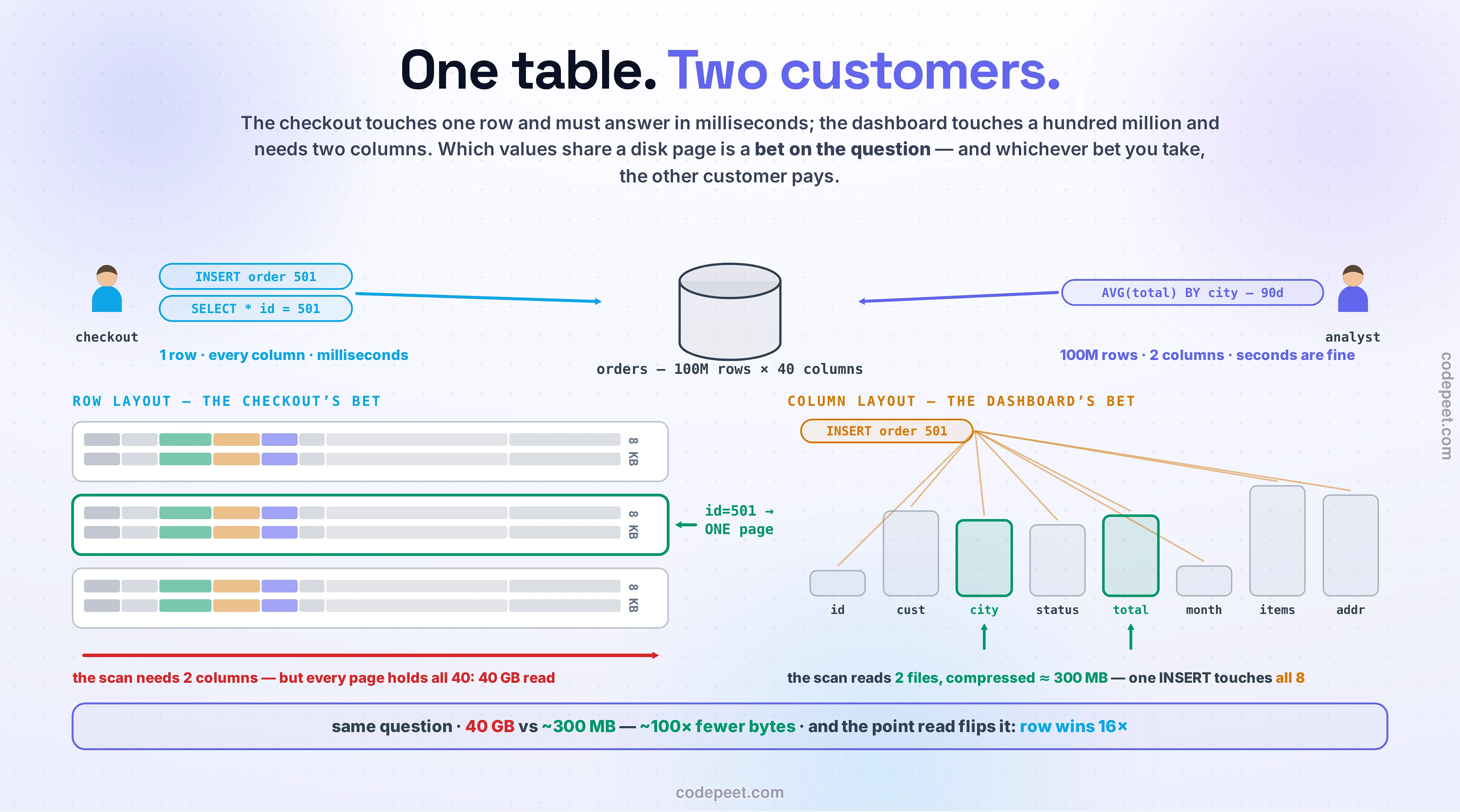
Read the first two lines again, because the whole lesson lives there. The checkout touches one row, every column. The dashboard touches every row, two columns. They're not asking bigger or smaller versions of the same question — they're asking questions with perpendicular shapes.

You've seen this movie eight times on the family map: the key-value store answers one shape instantly and fans out on everything else; the graph hops relationships and shards terribly; the search engine ranks words but can't do a transaction. Work is proportional to the question — and now that asymmetry shows up inside a single table, between two queries against the same rows.

One naming note before the physics, because it bites people in interviews: OLAP is a workload shape, not a product you buy. You can run analytics badly on your production Postgres tonight — nothing stops you except what's about to happen in the next section.

A disk doesn't hand you rows or columns. It hands you pages — fixed-size blocks (8 KB in Postgres), read whole. So somebody must decide, ahead of time, which values share a page. That decision is the entire fight.

The row bet. Store each order's forty fields side by side, orders packed one after another. Now "show me order 501" is a dream: the index walks to one page, and everything about order 501 comes up in a single read. An INSERT appends one row and touches a couple of indexes. This is why every OLTP engine you've met — Postgres, MySQL, and yes, Cassandra — stores rows together: the checkout's question shape is the layout.

Then the dashboard arrives. AVG(total) GROUP BY city needs two columns — but the pages don't contain columns, they contain orders. To read every total, the engine must drag every column of every row off disk. Run the arithmetic: 100 million orders × 40 fields ≈ a 40 GB table. Bytes the question actually needs: two columns ≈ 1.6 GB. The row layout forces you to read twenty-five times more than the question requires — before a single average is computed.

And no, an index doesn't save you. A B-tree is a machine for finding a few rows; visiting most of a table through an index means random hops that cost more than just reading it straight. The planner you met in Relational Databases: The Default for a Reason will weigh both plans and — correctly — pick the 40 GB sequential scan. The problem was never the plan. It's the layout.

The column bet. Flip the table ninety degrees: store all 100 million total values together in one file, all the city values in another, one file per column. The dashboard now reads exactly two files and ignores the other thirty-eight. Same disk, same table, same question — and the bytes read just fell from 40 GB to 1.6 GB, by rearrangement alone.

Then it gets better, twice —

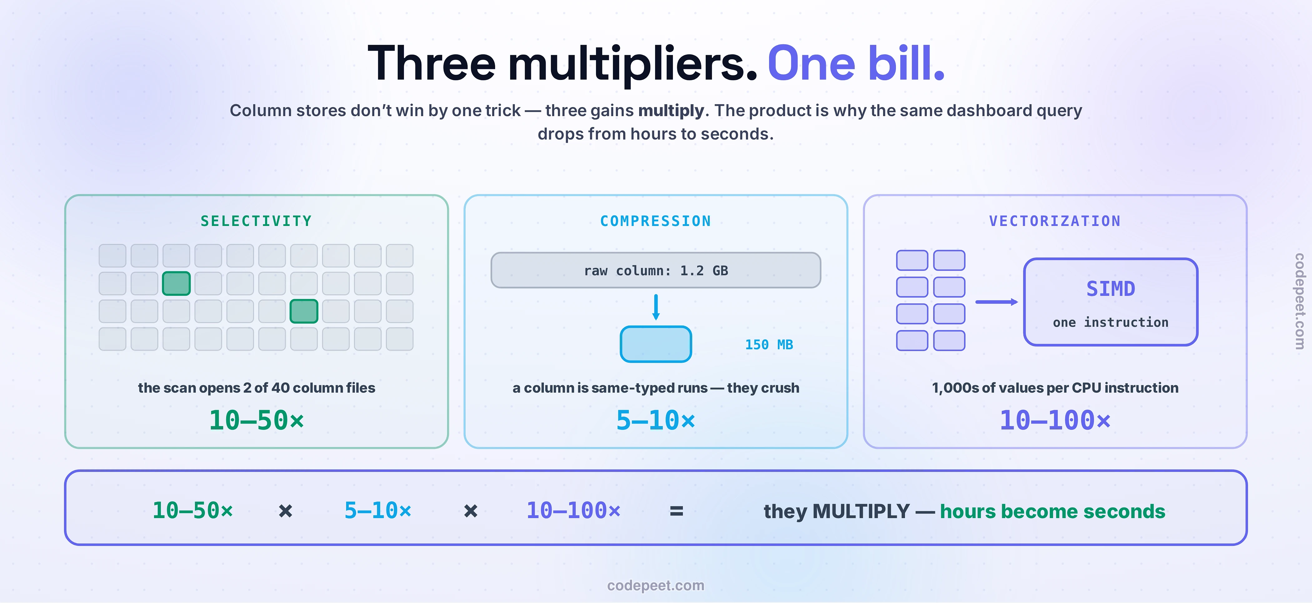
Multiplier one: selectivity. Read only the columns the question names. Two of forty ≈ 20× fewer bytes, straight off. (Typical published range: 10–50×, depending on how wide your rows are.)

Multiplier two: compression. A column file is a run of values of the same type with similar shapes — and that's exactly what compressors love. city has maybe 500 distinct values across 100 million rows: replace each string with a 2-byte dictionary code. status is even better: sorted runs of delivered, delivered, delivered… collapse under run-length encoding to "delivered × 3,180,442". Columnar engines routinely report 5–10× compression where row stores manage far less — a row is a grab-bag of types, and grab-bags don't compress. There's also a fixed tax that quietly disappears: row stores spend roughly 20 bytes of header per row (transaction visibility bookkeeping — the MVCC machinery); columnar files amortize their metadata across whole blocks. Our 1.6 GB of raw columns lands somewhere near 200–300 MB on disk.

Multiplier three: vectorization. Row engines traditionally process one row at a time — fetch, examine, advance — burning most of the CPU on the walking, not the math. Columnar engines feed the CPU dense batches of 1,024–2,048 same-typed values, and modern SIMD instructions apply one operation across a whole batch at once. On aggregations, that alone is worth 10–100×.

Stack them: 20× fewer bytes asked for, ~7× compression on what's left, then a CPU that averages thousands of values per step. That's how a query that ties up a production database for minutes finishes in well under a second on a columnar engine — arithmetic, not magic.

Now the bill. Store columns together and you've un-stored rows together. One INSERT now fans out to forty column files instead of appending one row. "Show me order 501" means visiting forty files and stitching the order back together — tuple reconstruction, the columnar world's version of the coat-check clerk searching every shelf. Updates? Compressed runs don't take kindly to edits; most columnar engines buffer changes and rewrite blocks wholesale.

So the trade is perfectly symmetric: row layout is a bet on the checkout's question; column layout is a bet on the dashboard's. Neither is smarter. They're the same data arranged for perpendicular questions — and whichever bet you take, the other customer pays. Feel both bets below: same table, both layouts, your queries, real byte counts.

Time to pay a debt. The wide-column lesson ended with a warning: wide-column is not columnar — the resolution comes one lesson later. This is that lesson.

Cassandra and Bigtable are row stores. A partition's rows live together, sorted by clustering key — that's the whole trick: hash to the cabinet, one sequential read inside the folder. Every cell of a row sits with its row. That is a write-optimized, OLTP-shaped bet, and calling the family "wide-column" is one of the great naming accidents of the field.

Columnar — what this lesson is about — is the opposite bet: one column's values across all rows stored together, for scanning. Snowflake, Redshift, ClickHouse, DuckDB, Parquet files in a lake: that world.

Same word, perpendicular physics. If an interviewer asks you to "use Cassandra for the analytics warehouse," you now know exactly which wire got crossed — and you can uncross it in two sentences.

One more echo you've already met: the time-series lesson compressed each metric's stream with delta-of-delta and XOR tricks — values of one kind, stored together, squeezed because neighbors resemble each other. That was columnar thinking wearing a time-series costume. The general form of that idea is this lesson.

Here's the incident, step by step, because you will meet it. The analyst — doing nothing wrong — points a BI tool at the production database and runs the 90-day dashboard. The engine begins its 40 GB sequential scan. Two things now happen to the checkout:

First, the buffer pool floods. The database keeps hot pages — tonight's active orders, the indexes checkout walks — cached in RAM. A whole-table scan shoves 40 GB through that cache and evicts the working set. Every checkout read that was a memory hit is suddenly a disk trip.

Second, the disks and CPU are busy serving the scan. The insert that used to take four milliseconds now queues. Checkout p99 spikes at exactly 9:04 AM every Monday, and nobody connects it to "Priya opened the revenue dashboard" until someone finally graphs the two together.

Notice what kind of failure this is: not a crash — an interference. Two workloads with opposite contracts sharing one buffer pool, one disk, one CPU. The latency-critical one always loses, because the scan-shaped one is, by nature, a bulldozer.

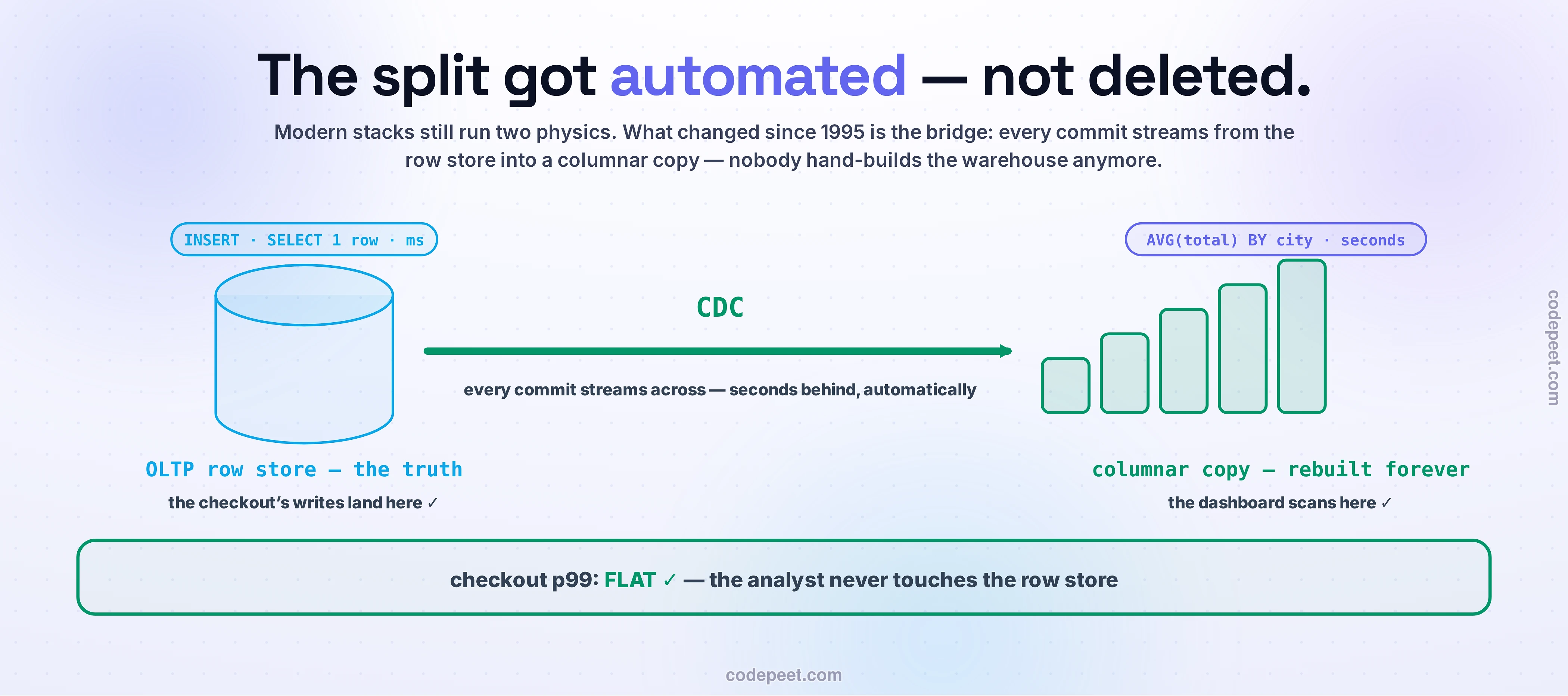
So the industry's answer, for forty years, has been blunt: separate them. The OLTP store stays the system of record — small, hot, guarded. Analytics gets a copy — in a columnar system built for scans — refreshed continuously or on schedule. The bridge between them is a pipeline: extract changes from the transactional store (change-data-capture — the mechanics live with delivery semantics and CDC in the fundamentals container), reshape, load. The whole discipline of ETL vs ELT and data pipelines, and the question of where the analytical copy should live — lakes, warehouses, lakehouses — gets its own act later in the course.

And here's the part that makes the split organizationally honest: the copy is allowed to be stale. The dashboard didn't need this morning's orders — it needed 90 days of history by 9:30. Declaring "analytics may lag by five minutes" is a design decision that buys you complete blast-radius isolation: Priya can run anything, and checkout will never feel it. OLTP is the business running; OLAP is the business learning — different teams, different tools, different truths about freshness. The split was never just about disks.

The vocabulary is older than you'd guess, and its history is funnier.

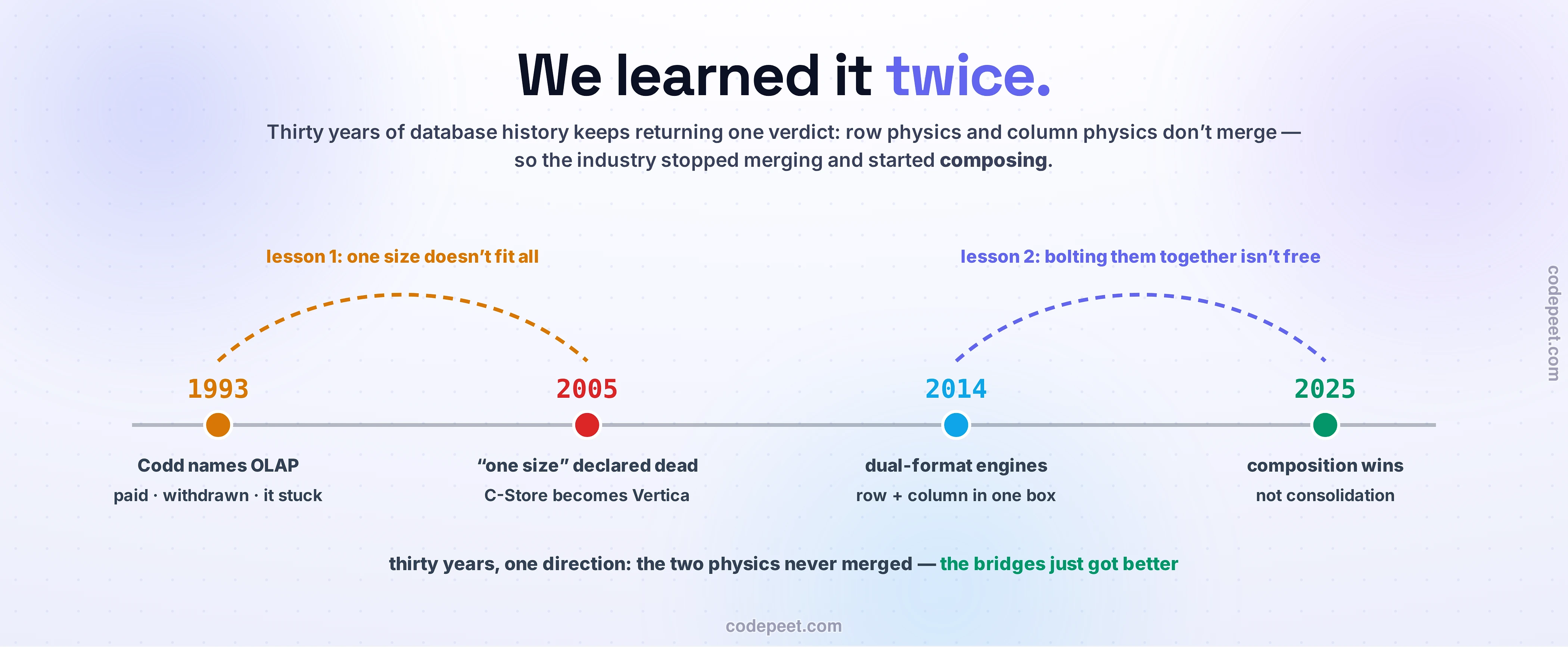
1993. E. F. Codd — yes, the same Codd whose relational bargain opened this section — publishes "Providing OLAP to User-Analysts: An IT Mandate," coining OLAP. The twist: the paper was a paid consulting piece for Arbor Software, whose Essbase product it conveniently blessed, and when Computerworld discovered the sponsorship it withdrew the paper. The name survived the scandal — because the workload split it named was real, even if the paper was marketing. The man who named the transactional era also named the analytical one; the second time, for money.

2005. Michael Stonebraker and Uğur Çetintemel publish "One Size Fits All": An Idea Whose Time Has Come and Gone — the paper this course's opening lesson leaned on. Prediction: the single do-everything DBMS fractures into specialized engines. That same year Stonebraker's group ships C-Store, the academic columnar engine that becomes Vertica; across the Atlantic, MonetDB/X100 works out vectorized execution. The two multipliers you just learned have separate birth certificates — layout-and-compression from C-Store, batch-at-a-time CPU work from X100.

2014. The one-box counterattack: Oracle ships Database In-Memory — the same table maintained twice, row format for transactions, in-memory column format for analytics, both kept in sync. The dual-format idea that every "translytical" system since has riffed on.

2024. The Stonebraker–Pavlo retrospective closes the loop with a sentence worth quoting verbatim: "The change to columnar storage revolutionized OLAP DBMS architectures." Every warehouse vendor converted. On the transactional side, meanwhile, the row store remains undefeated — for exactly the physics you now own.

So can't somebody just build one engine that loves both? People built them. HTAP — hybrid transactional/analytical processing — was a whole product category: SingleStore fused a rowstore with a columnstore; TiDB bolted a columnar replica onto a transactional core. The engineering worked. The market verdict, delivered in a widely-cited 2025 essay titled "HTAP is Dead": the category failed anyway — partly because most transactional apps fit comfortably on a single Postgres, and partly for the organizational reason you already know: product teams own OLTP, data teams own OLAP, and one box can't serve two owners. The essay's summary line is the honest one: "It's still HTAP — but through composition instead of consolidation."

Composition looks like this in 2026:

Zero-ETL — the cloud vendors automating the bridge. Aurora streams changes into Redshift's columnar world without a pipeline to babysit; the pattern is CDC-as-a-checkbox. The two systems remain two systems — you just stop hand-rolling the plumbing between them.

Dual-format engines — Oracle's In-Memory line, Google's columnar engines for AlloyDB and Spanner: keep the row store authoritative, maintain a columnar shadow inside the engine, route queries by shape. One box, but the two layouts still exist — physics conceded, packaging changed.

The embedded surprise — DuckDB: a full columnar, vectorized OLAP engine that runs in-process, no server at all — SQLite's trick applied to analytics. It topped ClickBench (the standard analytical benchmark) in late 2025, and its Postgres extension pg_duckdb routes analytical queries to a DuckDB engine living inside your Postgres: the project's benchmarks show a representative TPC-DS query going from ~90 seconds native to ~137 milliseconds. Read that carefully: even inside one process, the speedup comes from switching to columnar layout and vectorized execution. The boundary between OLTP and OLAP got thin, cheap, and automatic — but it did not disappear. It can't. It's a layout decision, and every byte sits somewhere.

The near-future direction, for your radar and no more: transactional stores streaming into open columnar table formats on object storage — the lakehouse pattern, which the 2024 retrospective calls the OLAP archetype for the next decade. It gets its own lesson in Lakes, Warehouses, Lakehouse.

None of this means your seed-stage app needs a warehouse. It means you should know which rung you're standing on, and what pain moves you up one:

Rung 1 — one box. Dashboards query production Postgres. Completely fine while tables are small and analysts are polite. You are betting that no scan ever floods the buffer pool during peak checkout.

Rung 2 — a read replica. Point analytics at a replica: blast-radius solved — Priya can bulldoze all Monday and checkout never notices. Be honest about what this buys: isolation, not speed. The replica is the same row layout; the 40 GB scan is still a 40 GB scan, just on somebody else's disk.

Rung 3 — columnar, in place. A DuckDB/pg_duckdb sidecar, or a columnar extension: the layout fix without new infrastructure. This rung carries small teams shockingly far now.

Rung 4 — a real analytical copy. CDC out of the system of record into a columnar warehouse or lakehouse; declared staleness; the data team owns it. This is the composition pattern, and everything about building it — the pipelines, the destinations, batch versus streaming refresh — is where the course's big-data act picks up this thread (Batch vs Stream opens by leaning right back on this lesson).

The skill being trained here isn't picking rung 4 — it's naming the workload before picking anything. "Is this question OLTP-shaped or OLAP-shaped, how stale may the answer be, and whose p99 pays if I guess wrong?" Answer those three and the infrastructure picks itself.

You now hold the last piece of physics this section needed. The map gave you eight families; this lesson gave you the axis that cuts underneath all of them — every store on the map lives on one side of the row/column bet, and now you can see which and why. Next: the flame war you've been promised — SQL vs NoSQL — settled the boring way, with a checklist.