B-Trees & B+ Trees

Last lesson left a loose thread. When the executor needed order #501, it found that one row's page among millions in microseconds — and we said that's an index doing its quiet work and moved on. Time to pull the thread.

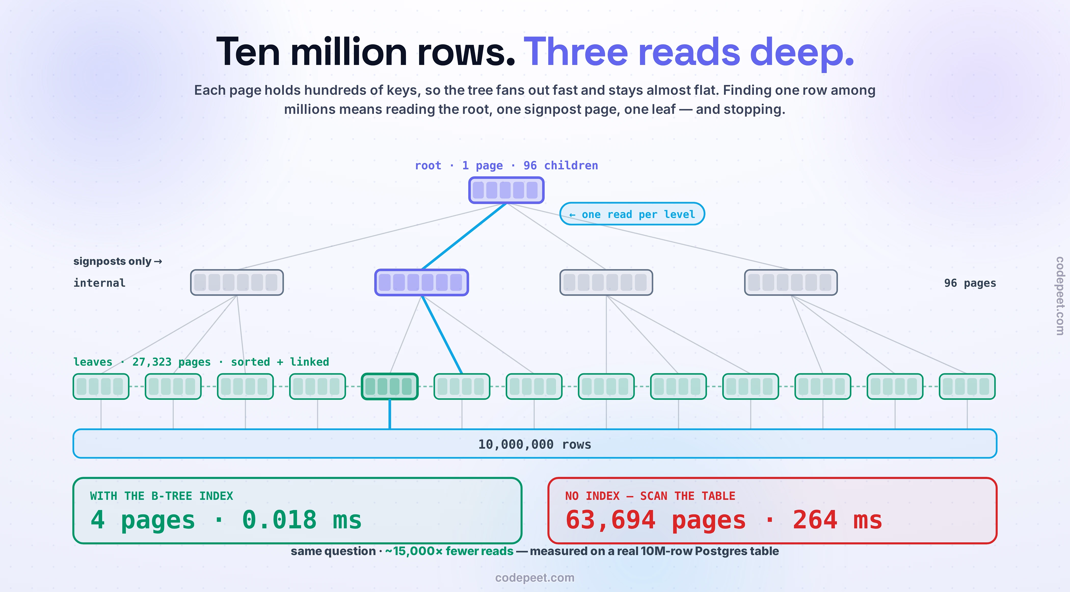
Here's the stakes, measured on a real table of ten million orders. Ask for one row by its id the slow way — no index — and Postgres reads 63,694 pages and takes 264 milliseconds, because it has no choice but to scan the whole 498 MB table looking for a match. Ask the same question with a B-tree index on id, and it reads 4 pages and takes 0.018 milliseconds. Same answer. Fifteen thousand times fewer reads.

That gap is the most important structure in databases, and it has a shape. This lesson builds it from scratch — why it's a tree, why the tree is absurdly wide and only three levels tall, what happens when you insert a key into a full node, and why the exact design that makes reads this fast makes some writes quietly expensive.

Start with the obvious idea and watch it break. Keep the ids sorted, then binary-search: 10 million rows is only ~23 halvings, so 23 probes and you're there. On paper, lovely.

On a disk, a disaster. Binary search jumps to the middle, then a quarter, then an eighth — each jump landing on a different, random 8 kB page. Every probe is a fresh page fetch, and 23 scattered fetches is 23 chances to wait on storage. Binary search is optimal for comparisons and terrible for page reads, which is the only cost that matters once data lives on disk.

The fix is one idea: stop splitting the search two ways. Split it hundreds of ways. If a single page you read can tell you which of 600 ranges your key falls into, you eliminate 599/600ths of the data with one read instead of half of it. Do that a second time and you've narrowed 10 million rows to a handful. That's a B-tree: a binary search's smarter, wider cousin, designed so that one page read makes an enormous decision.

A B-tree is built from pages — the same 8 kB pages from last lesson — wired into levels. Nearly every database index is really a B+ tree, and the plus is the part that matters, so let's build that one.

Leaf pages sit at the bottom and hold the real index entries: each key paired with a pointer to where the row actually lives (in Postgres, a tuple id — the heap page and slot number). The leaves hold every key, in sorted order, and — this is the B+ tree's signature — each leaf is doubly-linked to its neighbors. That linked list is why ORDER BY id and WHERE id BETWEEN 400 AND 500 are cheap: find the start, then walk sideways along the leaves, no tree-climbing required.

Internal pages above them hold no row data at all — only separator keys and pointers to child pages. They're signposts: keys < 5000 that way, 5000–10000 this way. Because an internal page spends all its space on signposts instead of data, it can point to hundreds of children. That single design choice — data only in the leaves, signposts up top — is the whole reason the tree stays short. (A classic B-tree stores data in the internal nodes too; that's why real databases use the B+ variant instead.)

Here is the number that makes databases possible. An 8 kB page, filled with small keys and child pointers, holds a few hundred of them. Call it a fanout of ~600. Then:

• 1 root page points to ~600 pages,
• each of those points to ~600 more — that's ~360,000 pages,
• each of those points to ~600 leaves — over 200 million entries.

Three levels. To find any one key among two hundred million, you read the root, read one child, read one leaf — three page reads, because at each level you only ever visit one page. The tree is a pancake: unimaginably wide, almost flat. Postgres's own documentation notes that over 99% of all pages in a B-tree are leaf pages — the navigation structure on top is a rounding error.

This isn't a whiteboard estimate. On our real 10-million-row table, the primary-key index has exactly this shape:

Add rows and the tree barely notices. Ten million rows: three levels. A hundred million: still three, maybe four. The height grows like the logarithm of your data — which is a mathematician's way of saying it basically doesn't grow at all. This is the answer to last lesson's cliffhanger, and it's why every serious database reached for the same structure.

A structure this tidy raises a fair question: how does it stay tidy as you insert millions of rows in random order? The answer is the single most important B-tree operation, and it's what you'll drive in a moment.

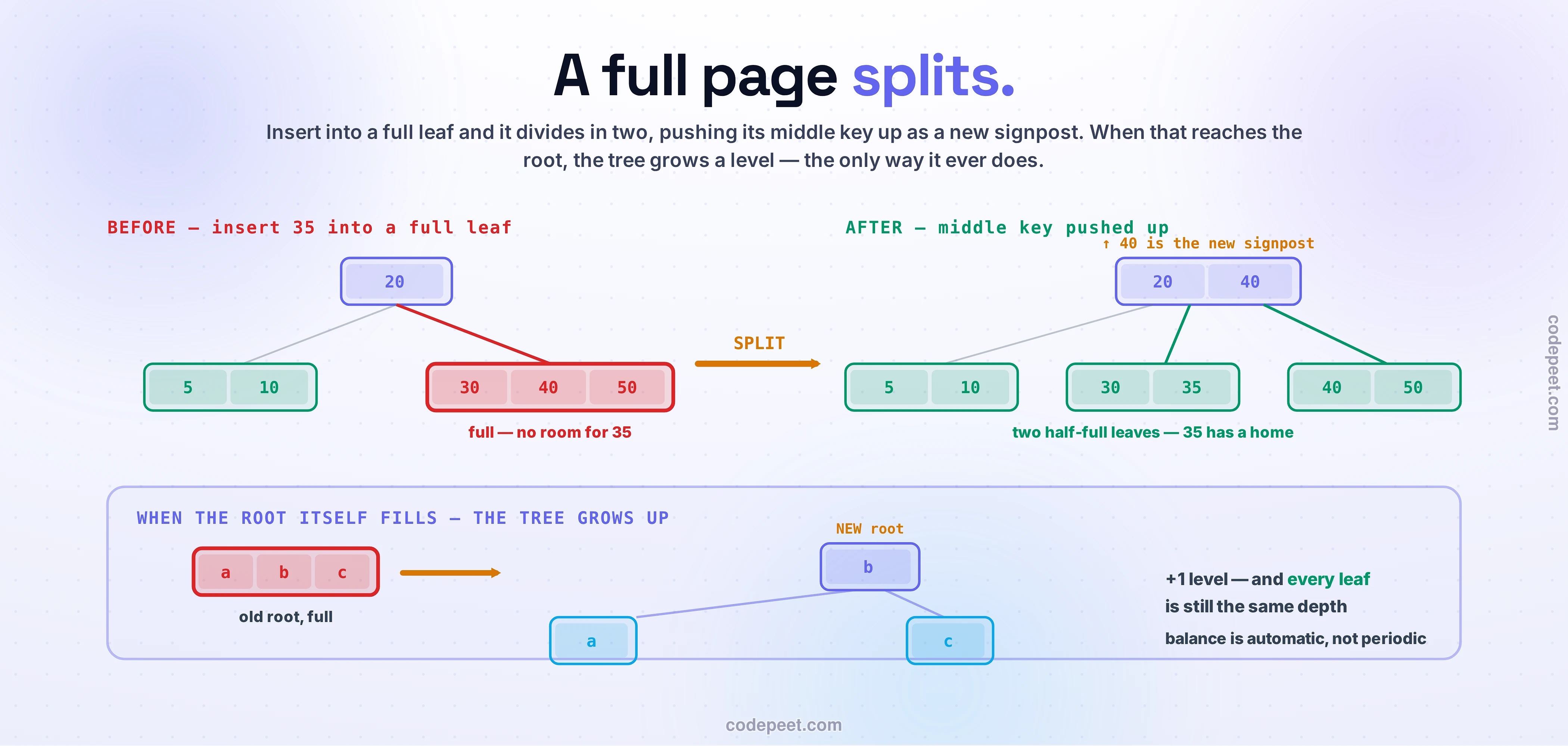
To insert a key, you descend to the leaf where it belongs and drop it into sorted position. Usually that's the whole story. But eventually a leaf is full — and here's the move: the leaf splits in two. Half the keys stay, half move to a brand-new sibling page, and the middle key is pushed up to the parent as a new signpost pointing at the new page.

Now the parent has one more entry. If it was full, it splits too, pushing its middle key up — a split can cascade all the way to the top. And when the root itself splits, the tree gains a level: a new root is created above the old one. That is the only way a B-tree ever gets taller, and it happens from the top down, which is precisely why the tree stays perfectly balanced — every leaf is always the exact same distance from the root. No leaf is ever deeper than another. The structure heals itself on every insert.

Here is the tree as a machine you can drive. Insert keys one at a time — type a value, or hit + sequential to append climbing keys, or + random to scatter them — and watch the descent path light up, a full leaf split in two, and the middle key climb toward the root. When the root itself splits, the whole tree gains a level in front of you, and the balanced? meter never once says no.

Try this first: hit + sequential a half-dozen times and watch a leaf fill, split, and push a key up. Then change the fanout dial from 4 down to 2 and watch the exact same keys build a taller tree — that's the whole reason real pages are made to hold hundreds of keys instead of a few. The payoff line does the arithmetic: at a real fanout of 600, a tree only this tall would already index hundreds of millions of rows, and a lookup would still read one page per level.

Because the leaves are sorted and linked, one structure answers a whole family of questions without breaking a sweat:

• Point lookups — WHERE id = 501 — descend to the leaf, done in ~3 reads.
• Ranges — WHERE id BETWEEN 400 AND 500, WHERE created > '2026-01-01' — find the start, walk the linked leaves.
• Sorting — ORDER BY id is free; the leaves are already in order.
• Prefix matches — LIKE 'piz%' is a range in disguise (everything from piz to pi{). But LIKE '%zza' is not — there's no sorted prefix to seek to, so a B-tree can't help a leading wildcard (which is exactly why full-text search needs a different index entirely).
• Min/max — the smallest key is the leftmost leaf; the largest is the rightmost.

One thing it pointedly does not do is WHERE status <> 'paid'. A not-equal match means everything except one value — no contiguous range to seek — so the index sits it out and the engine scans. The rule underneath all of this: a B-tree is a sorted structure, so it shines on anything that maps to a contiguous slice of that order, and shrugs at anything that doesn't. (The other index shapes — hash, composite, covering, partial — and the art of choosing them get their own lesson in Indexes Deep-Dive.)

Everything that makes a B-tree a brilliant reader has a bill, and it comes due on writes.

Go back to the split. When you insert a key into a full leaf, the engine rewrites the whole 8 kB page — and if that's the first time the page has been touched since the last checkpoint, it writes the entire page image into the WAL too (the full-page-image tax from last lesson). One logical row, a cascade of physical writes. Now the key question: where do your inserts land?

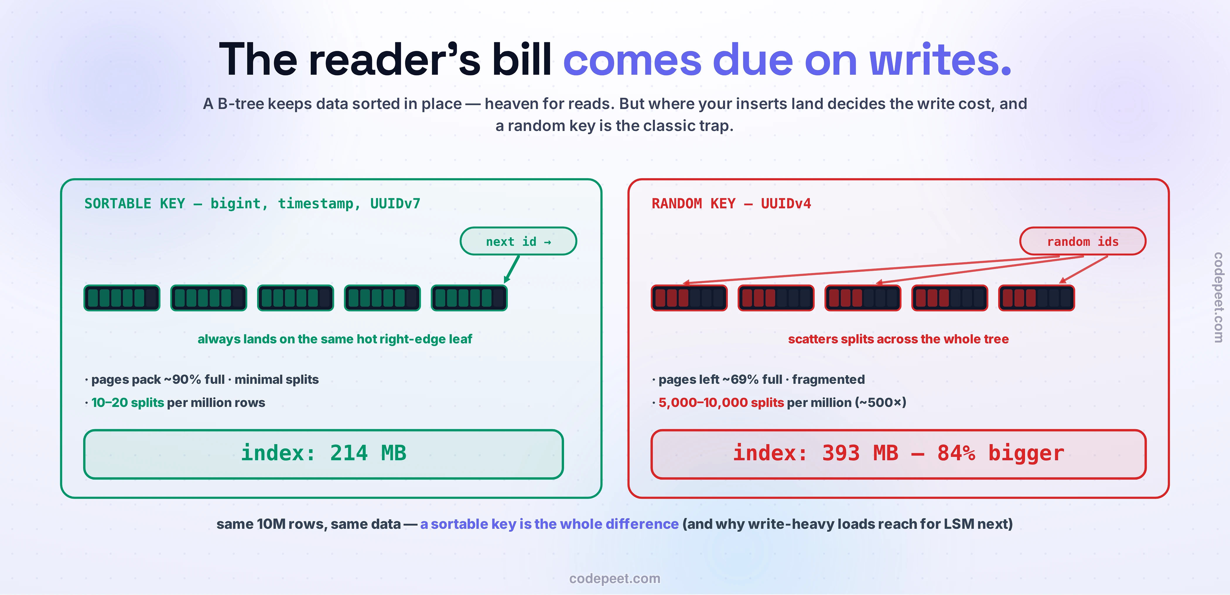
If your keys climb — a bigint that counts up, a timestamp, an auto-increment — every new key lands at the right edge of the tree, on the same hot leaf, which fills and splits cleanly and packs tight. Cheap. But if your keys are random — a UUIDv4 primary key is the classic trap — every insert lands on a different leaf somewhere in the middle, splitting pages all over the tree. The industry numbers are brutal: sequential keys cause 10–20 page splits per million rows; random UUIDs cause 5,000–10,000 — about 500× more — and leave leaves only ~69% full instead of packed. You saw the result yourself: the same ten million rows cost a 214 MB index on a bigint key and a 393 MB index on a random UUID — 84% larger, from nothing but insertion order. (The fix is a sortable key — a time-ordered UUIDv7, now native in Postgres 18 — so random-looking ids still land on the right edge.)

Step back and this is the whole personality of the structure. A B-tree keeps data sorted and in place, which is heaven for reads and range scans and murder for high-rate random writes. There's a law underneath: read, write, and space cost trade off against each other — you can only drive one down by pushing the others up. A B-tree spends write and space cost to buy cheap reads. Which raises the obvious question — what if your workload is the opposite, a firehose of writes you'll rarely read back? Then you want a structure that makes the other bet. That structure is the log-structured merge-tree, and it's next: LSM Trees & SSTables.

Every number in this lesson is reproducible in about ten minutes. This is the exact session (postgres:16 in Docker); the outputs are pasted from the real run.

1. Build ten million rows and look at the tree's actual shape.

2. Census every level of the index — see the pancake.

3. The whole point: index vs no index, same question.

Four pages versus sixty-three thousand. That is the entire reason indexes exist, on your screen.

4. Predict, then check: the random-key tax. Before you run this, guess which index will be bigger and by how much — the same ten million rows, one keyed by a counting bigint, one by a random UUID:

Clean up with docker rm -f <container> when you're done.

• "B-tree means binary tree." It doesn't. The B is not binary — a B-tree node is wide, fanning out to hundreds of children, not two. That width is the entire reason the tree is three levels tall instead of twenty-three. If you picture a binary tree, you've pictured the thing B-trees were invented to avoid.
• "An index stores a copy of the rows." It stores keys and pointers — like the index at the back of a book: the word and the page number, not the page. A B-tree leaf holds key → tuple id, and the executor follows that pointer to the heap. (The one exception: a clustered index, like an InnoDB primary key, keeps the row right in the leaf — worth knowing, covered in Indexes Deep-Dive.)
• "More indexes just make things faster." Faster to read, slower to write. Every index is another tree that must be descended, updated, split, and occasionally de-bloated on every insert and update. Three indexes means a write touches four structures. Indexes are a bet you place per query pattern, not free speed.
• "The database periodically rebuilds the tree to keep it balanced." No — it stays balanced by construction, on every single insert, through splits. Height only ever grows at the root, and every leaf is always the same depth. (You may still REINDEX to reclaim bloat from a random-key table — but that's compaction, not balancing.)
• "Huge tables mean deep trees." Real-world indexes are four or five levels deep even for hundreds of millions of rows; a depth of six is a curiosity. Logarithmic growth means the tree is, for all practical purposes, a constant three-or-four reads no matter how big your data gets.

• A B-tree index is a wide, shallow tree of pages: internal pages are signposts (keys + child pointers), leaf pages hold every key in sorted order paired with a pointer to the row.
• Fanout is the whole trick. Hundreds of children per page means millions of rows sit three or four levels deep — a lookup reads one page per level. Measured: 10M rows = 1 root → 96 internal → 27,323 leaves; a point query touched 4 pages / 0.018 ms versus 63,694 pages / 264 ms for a full scan.
• Inserts keep the tree balanced through splits: a full page splits and pushes its middle key up; the tree only grows taller when the root splits. Balance is automatic, not periodic.
• Because the leaves are sorted and linked, one index serves point lookups, ranges, ORDER BY, prefix matches, and min/max — but not <> or a leading %wildcard.
• It's a reader's structure. Random-key inserts (UUIDv4) scatter splits — ~500× more than sequential keys — bloating the index (measured 393 MB vs 214 MB); a sortable key (bigint, UUIDv7) keeps writes on the cheap right edge.
• That read-for-write bargain is a choice. When the workload is write-heavy, the opposite bet wins — the log-structured merge-tree of LSM Trees & SSTables, next.