Indexing Algorithms: HNSW & IVF

Introduction

Last lesson you learned that ANN trades a sliver of recall for a huge speedup. This lesson opens the two index structures that actually do it — the ones inside virtually every vector database: HNSW (a graph) and IVF (clustering).

You won't implement these — but understanding how they work pays off directly: it's what lets you pick the right one, tune its knobs (ef_search, nprobe — the recall dials from last lesson), and predict its memory and latency before you're surprised in production. Both rest on the same idea from last lesson — don't look everywhere, look only where the answer probably is — they just organize "where" differently.

In this lesson you'll learn:

HNSW — navigating a layered graph of neighbors
IVF — partitioning the space into searchable cells
Their memory / speed / scale tradeoffs, and which to choose
IVF-PQ for billion-scale, and the knobs that tune each

HNSW — Navigate a Graph of Neighbors

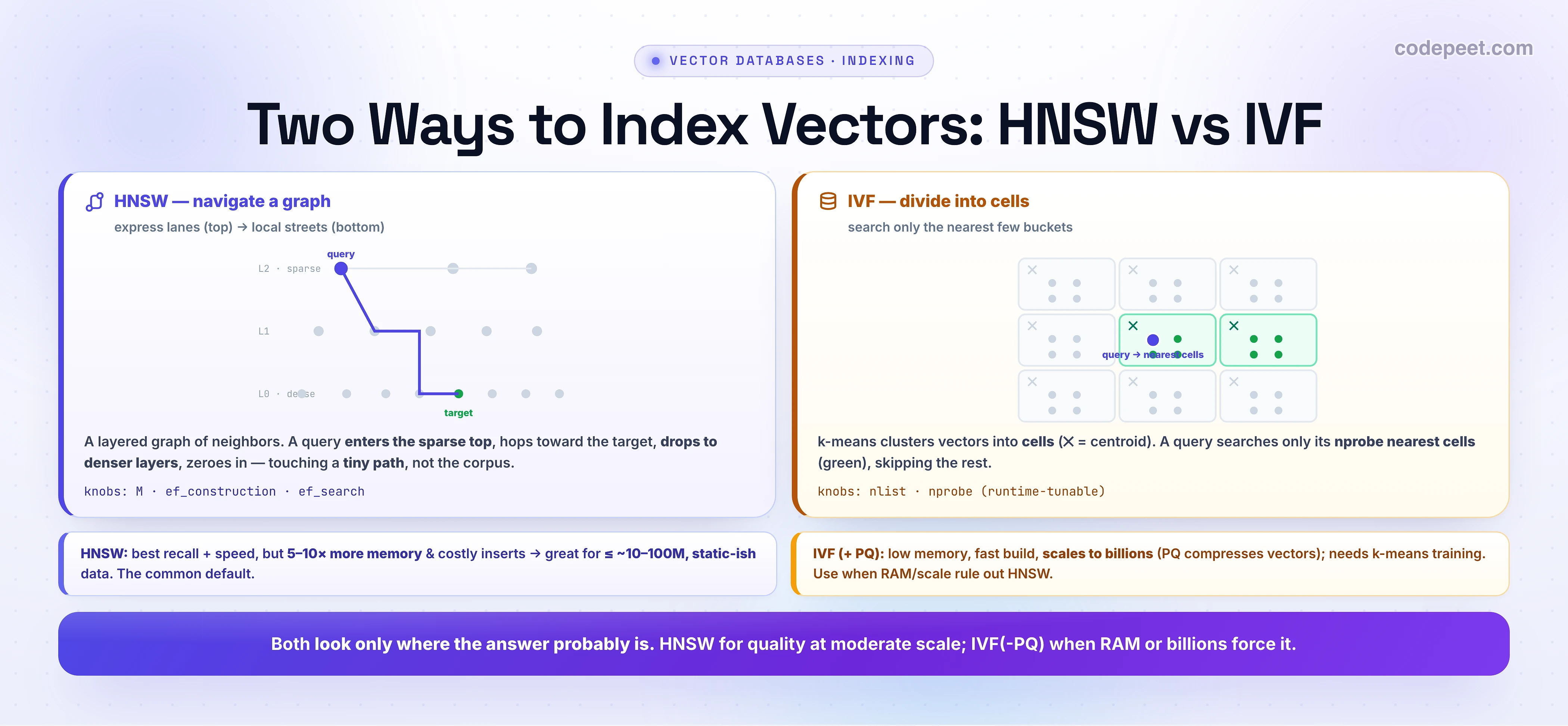
HNSW (Hierarchical Navigable Small World) is the most popular ANN index, and it works like a smart road network. Build a multi-layer graph where every vector is a node linked to its nearest neighbors:

Top layers are sparse — few nodes, with long-range links (think highways / express lanes).
Lower layers are dense — many nodes, short-range links (local streets).

A query enters at the sparse top and greedily hops toward the neighbor closest to the target. When no neighbor in that layer is closer, it drops down a layer (denser, finer) and continues — zooming in like driving the highway across the country, then exiting to surface streets near the destination. It visits only a tiny path of nodes, never the whole corpus — that's the sub-linear magic.

Knobs: M (links per node — higher = better recall, more memory), ef_construction (build effort/quality), and ef_search (the runtime recall↔speed dial — explore more of the graph for higher recall, slower).

An infographic titled 'Two Ways to Index Vectors: HNSW vs IVF' with two panels. The indigo HNSW panel (navigate a graph — express lanes at the top, local streets at the bottom) shows a three-layer graph: a sparse top layer L2, a middle layer L1, and a dense bottom layer L0; a query enters at the sparse top and a highlighted path hops across and drops down through the layers to reach the green target, touching only a tiny path, not the whole corpus; knobs are M, ef_construction, ef_search. The amber IVF panel (divide into cells, search only the nearest few buckets) shows a 3-by-3 grid of cells each with a centroid marked X; k-means clusters vectors into cells, and a query in the centre searches only its nprobe nearest cells (highlighted green) while skipping the rest; knobs are nlist and nprobe (runtime-tunable). Two tradeoff notes: HNSW gives the best recall and speed but uses 5 to 10 times more memory and has costly inserts, great for up to about 10 to 100 million static-ish vectors, the common default; IVF plus PQ has low memory, fast build, and scales to billions because PQ compresses vectors, but needs k-means training. A bottom banner: both look only where the answer probably is — HNSW for quality at moderate scale, IVF-PQ when RAM or billions force it.

IVF — Divide Into Cells, Search the Nearest Few

IVF (Inverted File index) takes the opposite, partition approach — like organizing a library by section. First, cluster all vectors with k-means into nlist cells, each summarized by a centroid; assign every vector to its nearest centroid (an "inverted list" per cell). Now a query doesn't scan everything — it finds the nprobe centroids nearest to it and searches only those few cells, ignoring all the rest.

If you have 1,000 cells and set nprobe = 16, you search ~1.6% of the corpus — a ~60× reduction. Two things to know:

It needs a training step (k-means must learn the centroids from a sample) before you add vectors.
Edge effect: a true neighbor sitting just across a cell boundary can be missed — raise nprobe to search more neighboring cells and recover it.

Knobs: nlist (number of cells — more = finer partitions) and nprobe (cells searched — the recall↔speed dial, and crucially runtime-tunable without rebuilding the index).

HNSW vs IVF: The Tradeoff

They solve the same problem with very different cost profiles:

	HNSW (graph)	IVF (cells)
Recall + speed	Best — top-tier, >95%	Good, depends on `nprobe`
Memory	High — stores the graph (5–10× more than IVF-Flat)	Low — just centroids + lists
Build	Slower; costly inserts	Fast; needs k-means training
Scale sweet spot	≤ ~10–100M, static-ish	Billions (with PQ)
Tuning	`M`, `ef_search`	`nlist`, `nprobe` (runtime)

The rule of thumb: HNSW for the best quality at moderate scale (it's the default in most vector DBs); IVF (especially IVF-PQ) when RAM or billion-scale rule HNSW out. Many systems even combine ideas. You'll rarely choose by hand from scratch — your vector DB exposes these as index options, and the next lessons show how.

IVF-PQ and Friends (Scaling to Billions)

At truly massive scale (>100M vectors), even IVF's full vectors are too much RAM — so you compress them. IVF-PQ combines IVF's cells with Product Quantization (the compression idea from L77): each vector is encoded into a handful of bytes, so a billion vectors fit in RAM that would otherwise be impossible. The cost is some recall — recovered, as always, by rescoring the top candidates with full-precision vectors (the coarse-to-fine pattern).

You'll also hear of:

DiskANN — keeps the index on SSD instead of RAM, for huge corpora on cheaper hardware.
ScaNN (Google), LSH, and newer quantization schemes (RaBitQ).

You don't need the internals — just the map: HNSW (graph) and IVF/IVF-PQ (cells + compression) are the two pillars, and everything else is a variation on prune the search space, then optionally compress.

See the Knobs in Code

FAISS exposes both indexes with their parameters — the same vectors, two index strategies:

import faiss, numpy as np
d = 768
X = np.random.randn(1_000_000, d).astype('float32'); faiss.normalize_L2(X)

# --- HNSW (graph) ---
hnsw = faiss.IndexHNSWFlat(d, 32)      # M = 32 links per node
hnsw.hnsw.efConstruction = 200         # build quality (memory/time vs recall)
hnsw.add(X)                            # builds the graph
hnsw.hnsw.efSearch = 64                # runtime recall <-> speed knob
hnsw.search(X[:1], 10)

# --- IVF (cells) ---
quantizer = faiss.IndexFlatIP(d)
ivf = faiss.IndexIVFFlat(quantizer, d, 4096)   # nlist = 4096 cells
ivf.train(X)                           # k-means to learn the centroids (REQUIRED)
ivf.add(X)
ivf.nprobe = 16                        # search 16 nearest cells (tune at runtime, no rebuild)
ivf.search(X[:1], 10)

# --- IVF-PQ (compressed, for billions) ---
ivfpq = faiss.IndexIVFPQ(quantizer, d, 4096, 64, 8)  # 64 sub-vectors x 8 bits = 64 bytes/vec
ivfpq.train(X); ivfpq.add(X); ivfpq.nprobe = 16

🧪 Try It Yourself

Walk an HNSW query in the stepper below — watch it enter the sparse top layer, hop toward the target, drop into denser layers, and arrive, touching only a handful of nodes.

Then choose the index for each case (HNSW, IVF, or IVF-PQ?):

2M chunks, need the best possible recall and low latency, plenty of RAM. → ?
800M product vectors, RAM is tight, can tolerate ~92% recall. → ?
50K docs in a prototype. → ?

→ 1: HNSW (best recall/speed; 2M fits in RAM comfortably). 2: IVF-PQ (compression makes 800M affordable; tune nprobe for recall). 3: neither — brute-force/flat is exact and instant at 50K (last lesson!). Match the index to scale + memory + recall.

Interactive: an ANN index navigator. One fixed field of 46 vectors and a single query are searched three ways via tabs. BRUTE-FORCE scans all 46 (100% examined, always exact). HNSW draws a k-nearest-neighbour graph and runs a greedy beam search from a far entry node, hopping toward the query and touching only a small explored subgraph; an ef_search slider widens the beam to explore more (higher recall, more examined). IVF partitions the points into six k-means cells (centroids shown as X) and searches only the query's nprobe nearest cells; an nprobe slider searches more cells. Live stats show the percentage of the corpus examined and whether the method found the true nearest neighbour (ringed), and the verdict explains a miss — HNSW getting stuck in a local neighbourhood, or IVF's cell-boundary edge effect — and how raising ef_search or nprobe recovers recall. The lesson made tangible: HNSW navigates a graph and IVF probes a few cells, both examine a tiny fraction of what brute-force does, and both expose a runtime recall dial. A 2-D teaching model of the real algorithms.

Mental-Model Corrections

"HNSW and IVF are basically the same." No — HNSW navigates a graph; IVF searches a few clusters. Different geometry, different memory profile.
"HNSW is always best." Best recall/speed, but it uses 5–10× more memory and has costly inserts — IVF(-PQ) wins when RAM or billion-scale is the constraint.
"You must rebuild to change recall." For IVF, nprobe is runtime-tunable (and HNSW's ef_search too) — no rebuild to trade recall for speed.
"IVF just works." It needs k-means training first, and watch the cell-boundary edge effect (raise nprobe).
"I implement these myself." You configure them — your vector database (next lessons) exposes HNSW/IVF/IVF-PQ as an index choice.

Key Takeaways

HNSW (graph): a layered neighbor graph — query enters the sparse top, hops, drops to denser layers, visiting a tiny path. Knobs M, ef_construction, ef_search. Best recall+speed but 5–10× more memory; sweet spot ≤ ~10–100M, static-ish. The common default.
IVF (cells): k-means clusters vectors into nlist cells; a query searches only its nprobe nearest cells. Knobs nlist, nprobe (runtime-tunable). Low memory, needs training, scales to billions with PQ.
IVF-PQ compresses vectors (L77's quantization) for >100M vectors in RAM; DiskANN puts the index on SSD.
Choose by scale + memory + recall: HNSW for quality at moderate scale; IVF(-PQ) when RAM/billions force it; flat for small corpora.
You configure, not implement — these are index options in your vector DB (next).