LoRA & QLoRA Explained

Introduction

Everything in this section has been building to this lesson. L192 told you to freeze the base and train a tiny adapter — now you'll learn exactly what that adapter is. LoRA (Low-Rank Adaptation) is the dominant PEFT method, the one behind almost every fine-tune you'll do, and QLoRA is what stacks the L191 quantization on top so even a 70B fine-tunes on a single GPU.

The beautiful part is how simple the core idea is — it's a few lines of math and ~10 lines of code. By the end of this lesson you'll be able to read LoraConfig(r=16, lora_alpha=32, ...) and know precisely what every argument does, why B starts at zero, and why the same trick lets you fine-tune a model 20× too big for your GPU. This is the technical climax of the mechanics section.

An infographic titled 'LoRA & QLoRA Explained', the fifth lesson of section two on fine-tuning mechanics and the dominant parameter-efficient method. LoRA, Low-Rank Adaptation, rests on the insight that the weight update during fine-tuning has low intrinsic rank: adapting to a narrow task does not require changing the model in every direction. So instead of learning a full update delta-W to a weight matrix W-zero of shape d-by-k, LoRA freezes W-zero and learns the update as a product of two thin matrices, B of shape d-by-r and A of shape r-by-k, where the rank r is much smaller than d or k. The adapted weight is W-zero plus alpha over r times B-A, and the forward pass is h equals W-zero-x plus alpha-over-r times B-A-x, where alpha is a scaling factor. A is initialized random Gaussian and B is initialized to all zeros, so the update is zero at step one and the model is unchanged until it learns. The parameter count drops from d-times-k to r-times-d-plus-k; for rank sixteen on a 4096-by-4096 matrix that is about a hundred-and-thirty-thousand trainable parameters instead of sixteen-point-seven million, roughly a hundred-and-twenty-seven times fewer, and overall under two percent of the model trains. Typical rank is four to sixty-four, alpha is set around twice the rank for a stable update magnitude, and LoRA is applied to the linear modules, often the attention query, key, value, and output projections or all linear layers. At inference the B-A product can be merged into W-zero for zero added latency, or kept as a tiny swappable adapter. QLoRA stacks quantization on top: it hosts the frozen base in 4-bit NormalFloat, applies double quantization to the quantization constants, and uses paged optimizers that spill optimizer state to CPU RAM, while keeping the LoRA adapters in 16-bit and de-quantizing to bf16 to compute, so a 70-billion model that needs about 140 gigabytes in fp16 fine-tunes in about 36 gigabytes on a single GPU. The takeaway is that LoRA replaces a giant weight update with two thin low-rank matrices, and QLoRA adds a 4-bit base so even the largest models fit.

The Insight: The Update Is Low-Rank

Start with a question: when you fine-tune, how much do the weights really change? The LoRA authors found the answer is "in a surprisingly small number of directions." The update to a weight matrix — call it ΔW — has low "intrinsic rank".

Intuitively: a giant pre-trained weight matrix already knows how to do almost everything. Nudging it toward your narrow task (a format, a tone, a domain) doesn't require changing it in all of its thousands of dimensions — just a few. And a matrix that only varies along a few directions is, by definition, low-rank — which means it can be written as the product of two much smaller matrices. That single observation is the whole trick.

The Decomposition: W₀ + (α/r)·BA

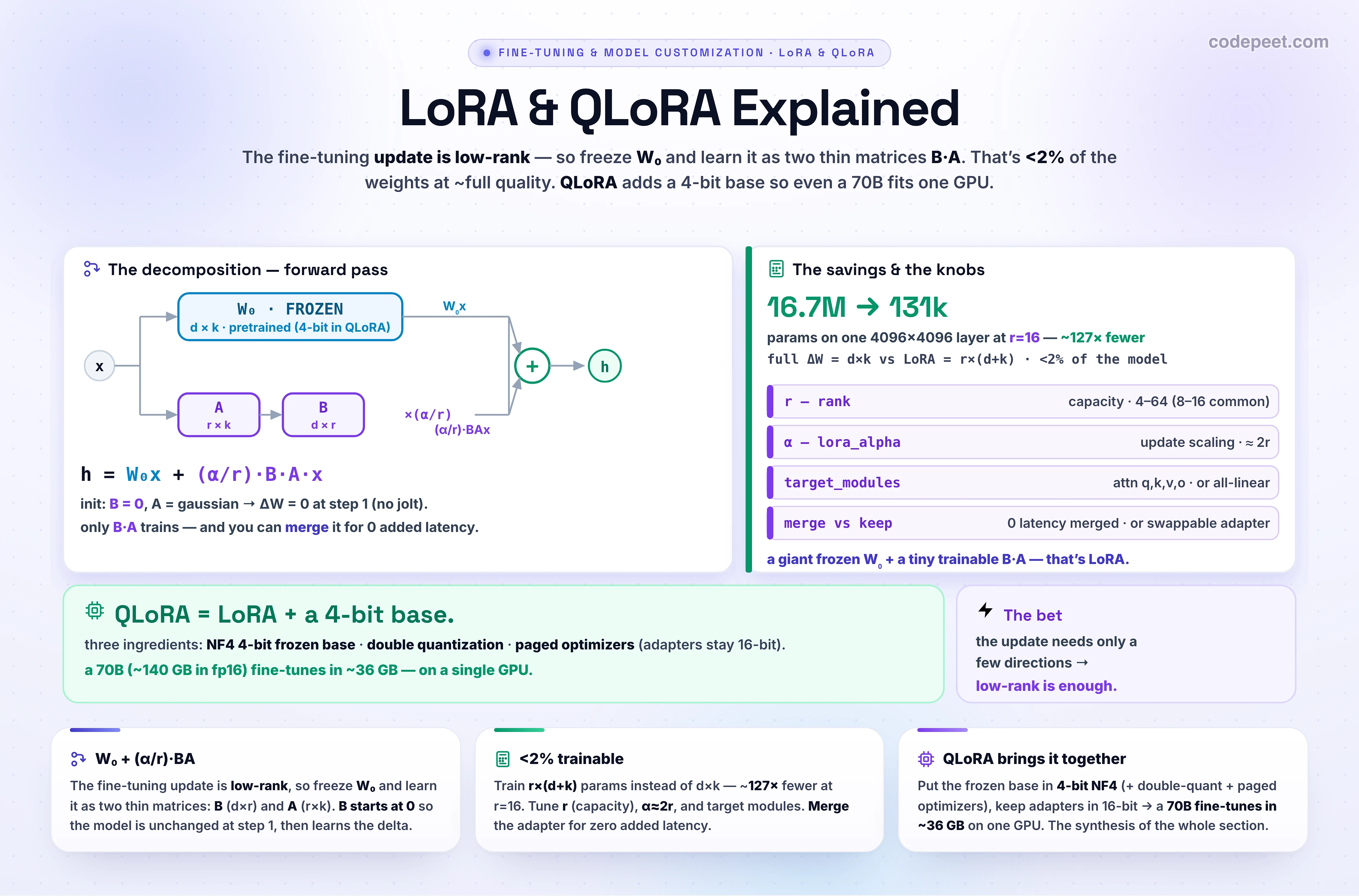
Full fine-tuning learns a full-size update ΔW (same shape as the weight W₀, say d × k). LoRA freezes W₀ and writes the update as a product of two thin matrices:

W = W₀ + ΔW = W₀ + (α/r)·B·A

where B is d × r, A is r × k, and the rank r ≪ min(d, k) (e.g. r=16 vs d=4096). Three details make it work:

Parameter count. You now train r × (d + k) numbers instead of d × k. For r=16 on a 4096×4096 matrix: 131k vs 16.7M — about 127× fewer, and <2% of the model overall.
The scaling (α/r). α (lora_alpha) scales the update; dividing by r keeps its magnitude stable as you change the rank. Rule of thumb: α ≈ 2r.
The initialization (the clever bit). A is random Gaussian, but B is all zeros — so ΔW = B·A = 0 at step 1. The model is identical to the pretrained one before training, then smoothly learns the low-rank delta. No disruptive jolt.

And the forward pass is just both paths added: h = W₀x + (α/r)·B·A·x. You'll see exactly this in the lab's arrow diagram.

The Knobs: r, α, target_modules & Merging

Four settings define a LoRA (you'll tune them in L194 (Fine-Tuning Hyperparameters & Tactics)):

r (rank) — the adapter's capacity. Higher r = more expressive (closer to full FT) but more params/memory. 4–64 is typical; 8–16 is the common default, larger only for harder tasks.
lora_alpha (α) — the update scaling, usually ≈ 2r.
target_modules — which weight matrices get an adapter. Classic is the attention q, k, v, o projections; all-linear (also the MLP) is common now for a bit more quality.
lora_dropout — light regularization on the adapter.

At inference you have a choice. Keep the adapter separate → it's a tiny swappable file (one base, many tasks — the L192 modularity win). Or merge it: compute W ← W₀ + (α/r)BA once, and the model runs at the exact same speed as the base — zero added latency, because there's no extra matrix at run time.

From Scratch: LoRA in ~10 Lines

LoRA isn't magic — it's a frozen Linear plus a trainable B@A. Here's the entire idea as a PyTorch module you could write yourself. (In practice you use the peft library, but seeing it bare is the point.)

import torch, torch.nn as nn

class LoRALinear(nn.Module):
    """A FROZEN Linear + a trainable low-rank update B@A. This is ALL LoRA is."""
    def __init__(self, base: nn.Linear, r=16, alpha=32):
        super().__init__()
        self.base = base                                  # the pretrained weight W0 - FROZEN
        for p in self.base.parameters():
            p.requires_grad = False
        d_out, d_in = base.weight.shape
        self.A = nn.Parameter(torch.randn(r, d_in) * 0.01)   # A: r x d_in   (random Gaussian)
        self.B = nn.Parameter(torch.zeros(d_out, r))         # B: d_out x r  (ZEROS -> dW = 0 at start)
        self.scale = alpha / r                               # the (alpha / r) scaling

    def forward(self, x):
        return self.base(x) + (x @ self.A.T @ self.B.T) * self.scale   # W0.x + (a/r).B.A.x

# Trainable params: r*(d_in + d_out)  instead of  d_in*d_out.
# For r=16 on a 4096x4096 layer:  131k  vs  16.7M  ->  ~127x fewer.
# Because B starts at 0, the model is UNCHANGED at step 1, then learns the low-rank delta.

QLoRA: Stacking 4-Bit on Top

QLoRA is the synthesis of this whole section: LoRA's low-rank adapter (L192/L193) on top of a 4-bit NF4 frozen base (L191). It adds three ingredients that together let a 70B — which needs ~140 GB in fp16 — fine-tune in ~36 GB on a single GPU:

4-bit NormalFloat (NF4) base — the frozen weights stored at 4 bits (the L191 lever), de-quantized to bf16 only for the forward-pass math.
Double quantization — quantize the quantization constants too, shaving a bit more.
Paged optimizers — spill optimizer state to CPU RAM during memory spikes (via unified memory) so you don't OOM.

Crucially, the LoRA adapters stay in 16-bit — high precision where the learning happens — so quality holds. In our stack it's one config object:

import torch
from transformers import AutoModelForCausalLM, BitsAndBytesConfig
from peft import LoraConfig, get_peft_model

# QLoRA = LoRA on a 4-bit NF4 FROZEN base. That's the whole trick.
qcfg = BitsAndBytesConfig(
    load_in_4bit=True,
    bnb_4bit_quant_type='nf4',                # 4-bit NormalFloat base (L191)
    bnb_4bit_use_double_quant=True,           # quantize the quant constants too
    bnb_4bit_compute_dtype=torch.bfloat16,    # de-quantize to bf16 to compute
)
base = AutoModelForCausalLM.from_pretrained('meta-llama/Llama-3.1-70B', quantization_config=qcfg)

lora = LoraConfig(r=16, lora_alpha=32, target_modules='all-linear', lora_dropout=0.05)
model = get_peft_model(base, lora)   # 16-bit trainable adapters on the 4-bit frozen base

# A 70B (~140 GB in fp16) now fine-tunes in ~36 GB - on a SINGLE 48GB GPU.
# Unsloth wraps this with ~2x speed + lower VRAM; Axolotl wraps it in a YAML config.

See It: The LoRA Lab

Build the decomposition by hand. Drag the rank r and watch the two thin matrices B·A grow and the trainable params (and savings) change in the forward-pass diagram. Then pick a dimension, switch target modules, and toggle QLoRA to watch the training memory collapse. Try r=4 (biggest savings, least capacity) vs r=128 (you're giving the savings back), and note how α=2r tracks along.

Interactive: the LoRA Lab. The user explores the low-rank decomposition at the heart of LoRA. They drag the rank r, pick the layer dimension d (1024, 4096, or 8192), choose the target modules (attention only versus all linear), and toggle QLoRA's 4-bit base. A forward-pass diagram with arrow connectors shows the two paths: the frozen W-zero on top and the trainable low-rank branch x into A into B times alpha over r, which merge at a sum node into the output h, with the matrix shapes labelled, B is d-by-r and A is r-by-d, and the thin matrices growing wider as the rank grows. Live math compares the full update delta-W at d-times-k parameters to LoRA at r times d-plus-k, the savings ratio of d over two r, the model-level trainable percentage, alpha which it sets to twice the rank, and the training memory which collapses further when QLoRA's 4-bit base is on, alongside a comparison to full fine-tuning. A verdict reacts to the rank: a low rank is the smallest adapter and biggest savings but less capacity, a mid rank is the common sweet spot with B starting at zero so the model is unchanged at step one, and a high rank adds capacity but gives back some of LoRA's savings.

That diagram is the lesson: a giant frozen W₀ plus a tiny trainable B·A — and QLoRA just makes the W₀ box 4-bit so the whole thing fits.

Why This Matters

LoRA + QLoRA is the way fine-tuning happens in 2026 — it's what every "fine-tune Llama on your data" tutorial, every Unsloth Colab, and every production adapter pipeline runs underneath. Understanding it from the matrix up means you can debug a run that won't fit (lower r, turn on QLoRA, target fewer modules), reason about quality-vs-cost (raise r for a hard task), and make the architecture call (merge for latency, or keep adapters swappable for many tasks). Every earlier lesson in this section — the loop, the memory math, quantization, PEFT — converges here, in a few thin matrices on a frozen, 4-bit base.

🧪 Try It Yourself

Compute the savings, then verify. For a 4096×4096 weight matrix at rank r=8: how many trainable parameters does LoRA add (r×(d+k)), versus full fine-tuning (d×k), and what's the ratio? Now open the LoRA Lab, set dim 4096 and r=8, and check. Then answer two design questions from the lab: (1) if your run is ~5 GB over your GPU, name three knobs that would shrink it; (2) why does B start at zeros and not random — what would break if both A and B were random? (Hint: what is ΔW at step 1?)

Mental-Model Corrections

"LoRA shrinks the model." No — the base is full size and frozen. LoRA adds a tiny trainable B·A beside it; only those few parameters train.
"A higher rank is always better." Higher r = more capacity and more params/memory; past a point it gives back LoRA's savings for little gain. 8–16 is the usual sweet spot.
"LoRA is slower at inference (extra matrices)." You can merge B·A into W₀ → identical speed to the base. The adapter only adds latency if you keep it separate (for swappability).
"QLoRA is a different method from LoRA." QLoRA is LoRA — just with the frozen base quantized to 4-bit (+ double-quant + paged optimizers). Same adapter math.
"The 4-bit base hurts quality a lot." The base is de-quantized to bf16 to compute and the adapters stay 16-bit, so QLoRA holds ~full-LoRA quality — for ~4× less memory.

Key Takeaways

LoRA's bet: the fine-tuning update is low-rank, so a full d×k change can be written as a thin B·A (rank r) — W = W₀ + (α/r)·B·A.
Tiny + safe: trainable params drop to r×(d+k) (~127× fewer at r=16/d=4096, <2% of the model), and B = 0 at init so the model is unchanged until it learns.
The knobs: r (capacity, 4–64), α ≈ 2r (scaling), target_modules (attn q,v,k,o or all-linear). Merge at inference for zero added latency, or keep it a swappable adapter.
QLoRA = LoRA + 4-bit: a NF4 frozen base + double-quant + paged optimizers → a 70B fine-tunes in ~36 GB on one GPU, with adapters in 16-bit so quality holds.
This is the default fine-tuning method in 2026 — the synthesis of the whole mechanics section.

Next: L194 — Fine-Tuning Hyperparameters & Tactics — how to actually choose r, α, learning rate, epochs, and batch size for a real run, closing Section 2.